We now look at an application of the Bayes rule that’s involves a continuous unknown random variable, which we try to estimate based on a discrete measurement.
Our model will be as follows.
We observe the discrete random variable K, which is Bernoulli, so it can take two values, 1 or 0.
And it takes those values with probabilities y and 1 minus y, respectively.
This is our model of K.
The catch is that the value of y is not known.
And it is modeled as a random variable by itself.
You can think of a situation where we are dealing with a single coin flip.
We observe the outcome of the coin flip, but the coin is biased.
The probability of heads is some unknown number, y.
And we try to infer or say something about the bias of the coin on the basis of the observation that we have made.
So what do we assume about this y or the bias of the coin? If we know nothing about this random variable, we might as well model it as a uniform random variable on the unit interval.
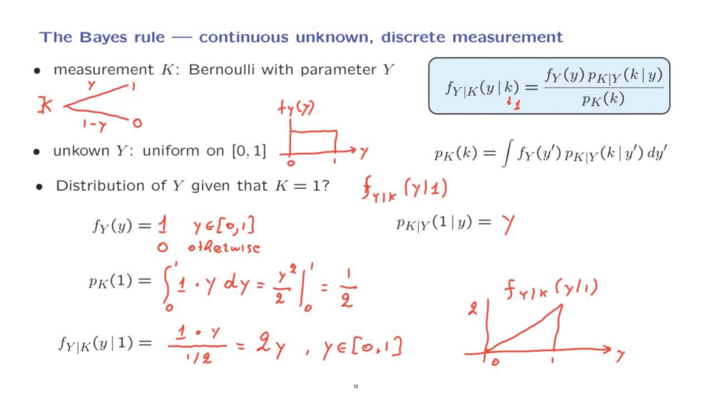
And the question now is, given that we made one observation and the outcome was 1, what can we say about the probability distribution of Y given this particular information? So the question that we’re asking is, what we can tell about the density of Y given that the value of 1 has been observed.
The way to approach this problem is by using a version of the Bayes rule.
We want to calculate this quantity for the special case where k is equal to 1.
So let us calculate the various pieces on the right hand side of this equation.
The first piece is the density of Y.
This is the prior density before we obtain any measurement.
And since the random variable is uniform, this is equal to 1 for y in the unit interval.
And of course, it is 0 otherwise.
The next piece that we need is the distribution of K given the value of Y.
Well, given Y, K takes a value of 1, with probability equal to Y– so the probability of 1, if we’re told the value of y is just a y itself.
y is the bias of the coin that we’re dealing with.
The next term that we need is the denominator.
We will use this formula.
It is the integral of the density of Y, which is equal to 1.
And it is equal to 1 only on the range from 0 to 1, times this probability that K takes a value, a certain value.
In this case, we’re dealing with a value of 1, so here we’re going to put 1 instead of k.
And therefore, we’re dealing with this expression here, which is just y.
And we integrated over y’s.
So this is y squared over 2, evaluated at 0 and 1, which gives us 1/2.
So this is the unconditional probability that K is equal to 1.
If we know nothing about Y, by symmetry, higher biases are equally likely as lower biases.
So we should expect that it’s equally likely to give us a 1 as it is to give us a 0.
Now, we have in our hands all the pieces that go into this particular formula.
And we can go ahead with the final calculation.
So in the numerator, we have 1 times this term, evaluated at k equal to 1, which is equal to y.
And then in the denominator, we have a term that evaluates to 1/2.
So the final answer is 2y.
Over what range of y’s is this correct? Only for those y’s that are possible.
So this is for y’s in the unit interval.
If we are to plot this PDF, it has this shape.
This is a plot of the PDF of Y given that the random variable K takes on a value of 1.
Initially, we started with a uniform for Y.
So all values of Y were equally likely.
But once we observed an outcome of 1, this tells us that perhaps Y is on the higher end rather than lower end.
So after we obtain our observation, the random variable Y has this distribution, with higher values being more likely than lower values.
This example is a prototype of situations where we want to estimate a continuous random variable based on discrete measurements.
Essentially it is the same as trying to estimate the bias of a coin based on a single measurement of the result of a coin flip.
As you can imagine, there are generalizations in which we observe multiple coin flips.
And this is an example that we will see later on in this class.