We have claimed that normal random variables are very important, and therefore we would like to be able to calculate probabilities associated with them.
For example, given a normal random variable, what is the probability that it takes a value less than 5? Unfortunately, there are no closed form expressions that can help us with this.
In particular, the CDF, the Cumulative Distribution Function of normal random variables, is not given in closed form.
But fortunately, we do have tables for the standard normal random variable.
These tables, which take the form shown here, give us the following information.
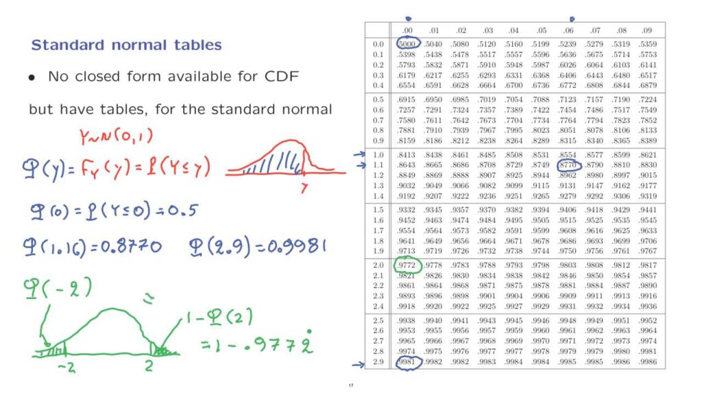
If we have a normal random variable, which is a standard normal, they tell us the values of the cumulative distribution function for different values of little y.
In terms of a picture, if this is the PDF of a standard normal and I give you a value little y, I’m interested in the corresponding value of the CDF, which is the area under the curve.
Well, that value, the area under this curve, is exactly what this table is giving to us.
And there’s a shorthand notation for referring to the CDF of the standard normal, which is just phi of y.
Let us see how we use this table.
Suppose we’re interested in phi of 0.
Which is the probability that our standard normal takes a value less than or equal to 0? Well, by symmetry since the PDF is symmetric around 0, we know that this probability should be 0.5.
Let’s see what the table tells us.
0 corresponds to this entry, which is indeed 0.5.
Let us look up the probability that our standard normal takes a value less than, let’s say, 1.16.
How do we find this information? 1 is here.
And 1.1 is here.
1.1, and then we have a 6 in the next decimal place, which leads us to this entry.
And so this value is 0.8770.
Similarly, we can calculate the probability that the normal is less than 2.9.
How do we look up this information? 2.9 is here.
We do not have another decimal digit, so we’re looking at this column.
And we obtain this value, which is 0.9981.
And by looking at this number we can actually tell that a standard normal random variable has extremely low probability of being bigger than 2.9.
Now notice that the table specifies phi of y for y being non-negative.
What if we wish to calculate the value, for example, of phi of minus 2? In terms of a picture, this is a standard normal.
Here is minus 2.
And we wish to calculate this probability.
There’s nothing in the table that gives us this probability directly, but we can argue as follows.
The normal PDF is symmetric.
So if we look at 2, then this probability here, which is phi of minus 2, is the same as that probability here, of that tail.
What is the probability of that tail? It’s 1, which is the overall area under the curve, minus the area under the curve when you go up to the value of 2.
So this quantity is going to be the same as phi of minus 2.
And this one we can now get from the tables.
It’s 1 minus– let us see, 2 is here.
It’s 1 minus 0.9772.
The standard normal table gives us probabilities associated with a standard normal random variable.
What if we’re dealing with a normal random variable that has a mean and a variance that are different from those of the standard normal? What can we do? Well, there’s a general trick that you can do to a random variable, which is the following.
Let us define a new random variable Y in this fashion.
Y measures how far away is X from the mean value.
But because we divide by sigma, the standard deviation, it measures this distance in standard deviations.
So if Y is equal to 3 it means that X is 3 standard deviations away from the mean.
In general, Y measures how many deviations away from the mean are you.
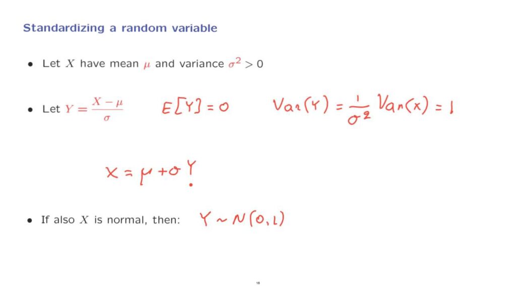
What properties does this random variable have? The expected value of Y is going to be equal to 0, because we have X and we’re subtracting the mean of X.
So the expected value of this term is equal to 0.
How about the variance of Y? Whenever we multiply a random variable by a constant, the variance gets multiplied by the square of that constant.
So we get this expression.
But the variance of X is sigma squared.
So this is equal to 1.
So starting from X, we have obtained a closely related random variable Y that has the property that it has 0 mean and unit variance.
If it also happens that X is a normal random variable, then Y is going to be a standard normal random variable.
So we have managed to relate X to a standard normal random variable.
And perhaps you can rewrite this expression in this form, X equals to mu plus sigma Y where Y is now a standard normal.
So, instead of doing calculations having to do with X, we can try to calculate in terms of Y.
And for Y we do have available tables.
Let us look at an example of how this is done.
The way to calculate probabilities associated with general normal random variables is to take the event whose probability we want calculated and express it in terms of standard normal random variables.
And then use the standard normal tables.
Let us see how this is done in terms of an example.
Suppose that X is normal with mean 6 and variance 4, so that the standard deviation sigma is equal to 2.
And suppose that we want to calculate the probability that X lies between 2 and 8.
Here’s how we can proceed.
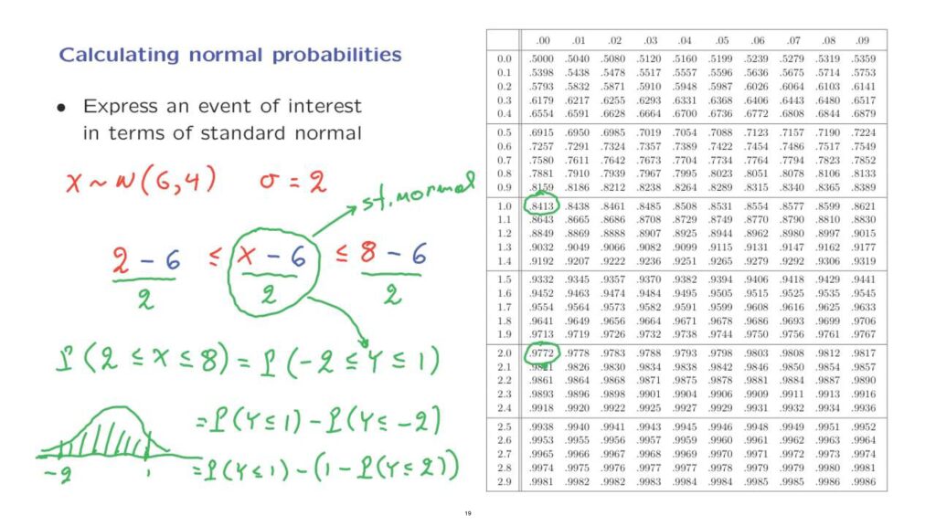
This event is the same as the event that X minus 6 takes a value between 2 minus 6 and 8 minus 6.
This event is the same as the original event we were interested in.
We can also divide both sides of this inequality by the standard deviation.
And the event of interest has now been expressed in this form.
But at this point we recognize that this is of the form X minus mu over sigma.
So this random variable here is a standard normal random variable.
So the probability that X lies between 2 and 8 is the same as the probability that a standard normal random variable, call it Y, falls between these numbers minus 4 divided by 2, that’s minus 2.
Then Y less than 1.
And now we can use the standard normal tables to calculate this probability.
We have here 1 and here we have minus 2.
And we want to find the probability that our standard normal falls inside this range.
This is the probability that it is less than 1.
But we need to subtract the probability of that tail so that we’re left just with this intermediate area.
So this is the probability that Y is less than 1 minus the probability that Y is less than minus 2.
And finally, as we discussed earlier, the probability that Y is less than minus 2, this is 1 minus the probability that Y is less than or equal to 2.
And now we can go to the normal tables, identify the values that we’re interested in, the probability that Y is less than 1, the probability that Y is less than 2, and plug these in.
And this gives us the desired probability.
Again, the key step is to take the event of interest and by subtracting the mean and dividing by the standard deviation express that same event in an equivalent form, but which now involves a standard normal random variable.
And then finally, use the standard normal tables.