In this lecture sequence, we introduced quite a few new concepts and went through a fair number of examples.
So for this reason, it is useful now to just take stock and summarize the key ideas and concepts.
The starting point in a Bayesian inference problem is the following.
There’s an unknown parameter, Theta, and we’re given a prior distribution for that parameter.
We’re also given a model for the observations, X, in terms of a distribution that depends on the unknown parameter, Theta.
The inference problem is as follows.
We will be given the value of the random variable X.
And then we want to find the posterior distribution of Theta, that is, given this particular value of X, what is the conditional distribution of Theta?
In the case where Theta is discrete, this will be in terms of a PMF.
If Theta is continuous, this would be a PDF.
We find the posterior distribution by using an appropriate version of the Bayes rule.
And here we have four different combinations or four choices, depending on which variables are discrete or continuous.
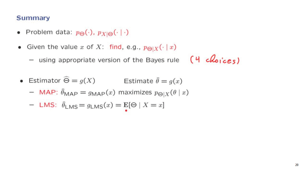
This is a complete solution to the Bayesian inference problem– a posterior distribution.
But if we want to come up with a single guess of what Theta is, then we use a so-called estimator.
What an estimator does is that it calculates a certain value as a function of the observed data.
So g describes the way that the data are processed.
Because X is random, the estimator itself will be a random variable.
But once we obtain a specific value of our random variable and we apply this particular estimator, then we get the realized value of the estimator.
So we apply g now to the lowercase x, and this gives us an estimate, which is actually a number.
We have seen two particular ways of constructing estimates or estimators.
One of them is the maximum a posteriori probability rule in which we choose an estimate that maximizes the posterior distribution.
So in the case where Theta is discrete, this finds the value of theta, which is the most likely one given our observation.
And similarly, in the continuous case, it finds a value of theta at which the conditional PDF of Theta would be largest.
Another estimator is the one that we call the LMS or least mean squares estimator, which calculates the conditional expectation of the unknown parameter, given the observations that we have obtained.
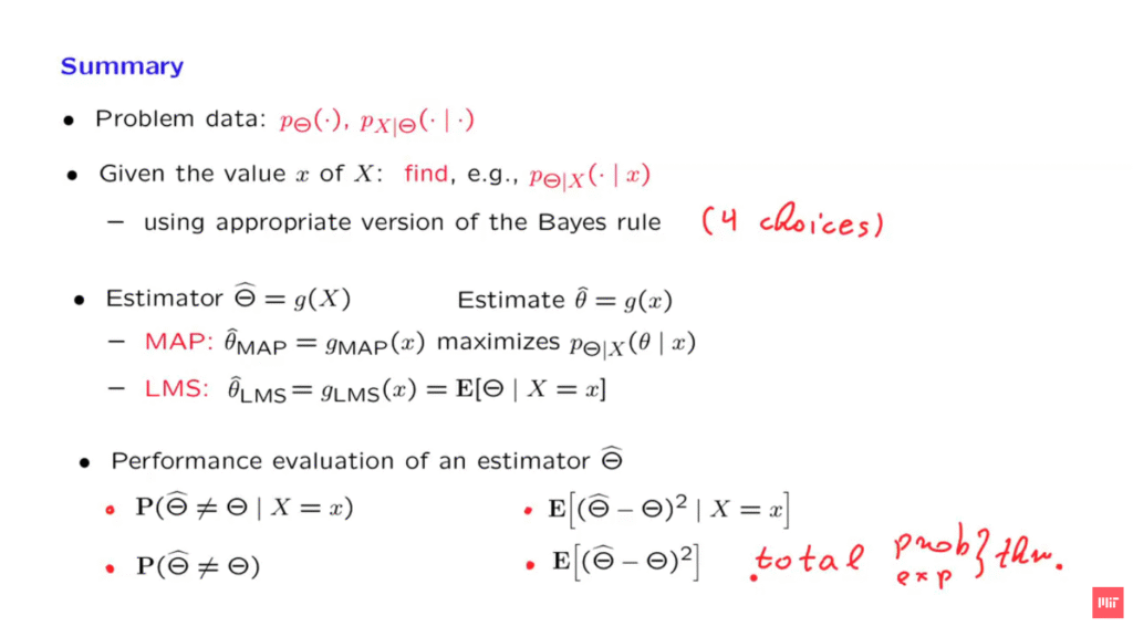
Finally, we may be interested in evaluating the performance of a given estimator.
For hypotheses-testing problems we’re interested in the probability of error.
And we have the conditional probability of error.
Given the data that I have just observed and given that I’m using a specific estimator, what is the probability that I make a mistake?
And then there’s the overall evaluation of the estimator– how well does it do on the average before I know what X is going to be?
And this is just the probability that I will be making an incorrect decision.
For estimation problems, on the other hand, we’re interested in the distance between our estimates from the true value of Theta.
And this leads us to the following conditional mean squared error, given that we have already obtained an observation.
And we come up with an estimator.
In particular, the value of the estimator at this time would be completely determined by the data that we obtained.
But Theta, the unknown parameter remains random.
And there’s going to be a certain squared error.
We find the conditional expectation of this squared error in this particular situation, where we have obtained a specific value of the random variable, capital X.
On the other hand, if we’re looking at the estimator more generally, how well it does on the average, then we look at the unconditional mean squared error, and this gives us an overall performance evaluation.
How do we calculate these performance measures?
Here, we live in a conditional universe.
And in a Bayesian estimation problem at some point we do calculate the posterior distribution of Theta, given the measurements.
So these calculations involved here consist of just an integration or summation using the conditional distribution.
For example, here we would integrate this quantity using the conditional density of Theta, given the particular value that we have obtained.
If we want to now calculate the unconditional performance, then we would have to use the total probability or expectation theorem.
And in that case, we can average over all the possible values of X to find the overall error.
So all of the calculations involve tools and equations that we have seen and that we have used in the past, so it is just a matter of connecting those tools with the specific new concepts that we have introduced here.