We will now go through another example to consolidate our intuition about the content of the law of iterated expectations and the law of the total variance.
The example is as follows.
We have a class, and that class consists of 30 students in total who are divided into sections– the first and the second section.
Let xi be the score of students i, let’s say the final grade in the class.
We consider the following probabilistic experiment.
We pick a student at random, uniformly, so that each student is equally likely to be picked.
And we define two random variables– X is a numerical random variable that gives us the score of the selected student.
So if student i is selected, the value of the random variable capital X is xi.
And capital Y is defined as the random variable, which is the section of the selected student, so that y takes values 1 or 2.
We’re given some information.
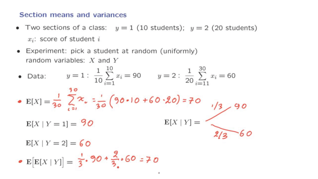
For the first section, the average of the student scores is 90.
For the second section, the average of the student scores is 60.
Given that information, what is the expected value of the student score?
Well, each student is equally likely to be picked, so has probability 1 over 30 to be picked.
And this multiplies the score of the student, so this is the expected value of the random variable of interest.
What is this number?
Well, we need to calculate the sum of the xi’s.
The sum of the first 10 xi’s is equal to 90 times 10, and the sum of the xi’s in the other section is equal to 60 times 20.
And we carry out the calculation, and we find that the answer is 70.
Now let us look at conditional expectations.
If Y is equal to 1, this means that a student from section one was picked.
And within that section, each student is equally likely to be picked, so the outcome of this random variable is equally likely to be any one of these xi’s.
Each xi gets picked with probability of 1 over 10.
And so, the expected value of this random variable is 90.
Similarly for the second section, the expected value of the score of a randomly selected student, given that the student belongs in that section, is equal to 60.
With this information available, now we can describe the abstract conditional expectation, which is a random variable.
This random variable takes the value of 90 if a student from the first section was picked, and the value of 60 if a student from the second section was picked.
What is the probability of this event that the student from the first section was picked?
Given that the first section has 10 out of a total of 30 students, this probability is 1/3, and therefore, this probability is 2/3.
Now that we have the distribution of this random variable, we can calculate the expected value of this random variable, which is 1/3 times 90 plus 2/3 times 60.
And this number evaluates to 70, which of course, it’s no coincidence, it’s the same as the average over the entire class.
By the law of iterated expectations, we know that this quantity should be the same as this quantity.
So the law of iterated expectations allows us to calculate the overall average in the entire class by taking the section averages, and weigh them according to the sizes of the different sections.
It’s a divide and conquer method, and it is similar to what we have been doing when we use the total expectation theorem to divide and conquer.
We continue with our example, and here is a summary of what we found so far.
The conditional expectation is a random variable that takes these two values with certain probabilities.
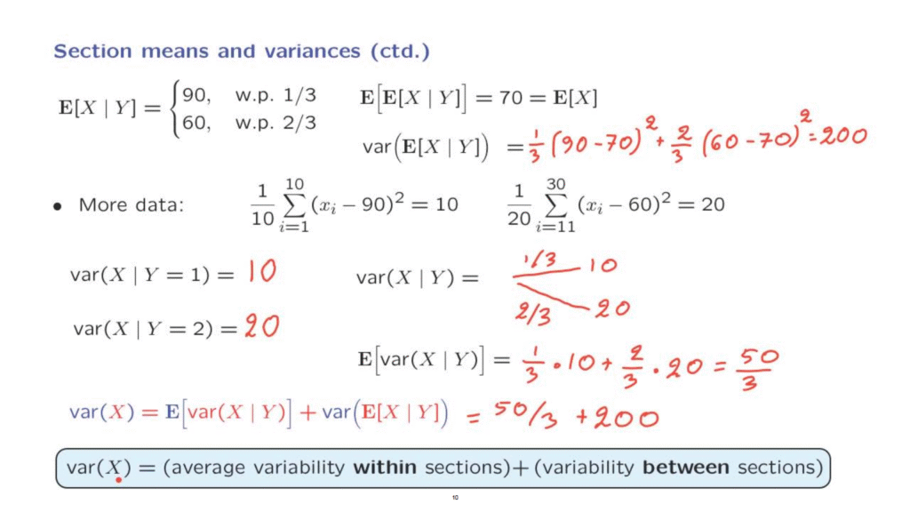
And the mean of this random variable is equal to 70.
Let us now calculate the variance of this random variable.
This random variable, with probability 1/3, takes a value 90, which is this much away from the mean of this random variable, which we square.
And with probability 2/3, it takes a value of 60, which is this much away from the mean of the random variable.
We square this, as well.
And when we carry out the calculation, we find that this number is equal to 200.
Let us now continue.
And suppose that somebody gave us this piece of information.
For the first section, this is the deviation of the i-th student from the mean of that section.
So this is the sum of the squares of the deviations and then we average over all the students.
We will use this data to calculate certain quantities– for example, the variance of the scores in the first section.
Now in the first section, with probability 1/10, we pick the ith student that has this score.
And this is the deviation of that student from the mean of that section.
So this is the same as the mean squared deviation from the mean of the section.
And this is exactly the variance within that section.
It is the variance of the random variable, which is the score of a random student, given that we are selecting a student from the first section.
For the second section, the story similar.
We’re given this information, and this tells us the variance of the student scores within the second section.
So now we can describe the abstract conditional variance.
It is a random variable that takes this value with probability equal to the probability of selecting someone from this section, which is 1/3.
Or it takes a value of 20, which is the variance in the second section.
And the second section is selected with probability 2/3.
With this information at hand, now we can calculate the expected value of this random variable, which is 1/3 times 10 plus 2/3 times 20, which is 50/3.
At this point, we have the two quantities that are necessary to apply the law of total variance.
According to the law of total variance, the variance of the student scores throughout the entire class is equal to this number, which is 50/3, plus this number, which is 200.
And this is the overall variance.
Now let us interpret the law of total variance in this context.
The interpretation is as follows.
The variance of the student scores in the entire class consists of two pieces.
The first piece looks at the variance inside each section, which is 10 or 20, depending on which section we’re looking at.
And we take the average over the different sections.
So we look at the variability of the scores within a typical section, and then we average over all the sections.
The other term looks at the means in the different sections, and figures out how different are these means.
How much do they vary from the overall class average?
It measures the variability between different sections.
So the overall randomness in the test scores can be broken down into two pieces of randomness.
One source of randomness is that the different sections have different means.
The other source of randomness is that inside each section, the students are different from the means of their section.
And these two pieces of randomness together add up to the total randomness of the student scores as measured by the variance of the entire class.