As a warm-up towards finding the distribution of the function of random variables, let us start by considering the discrete case.
So let X be a discrete random variable and let Y be defined as a given function of X.
We know the PMF of X and wish to find the PMF of Y.
Here’s a simple example.
The random variable X takes the values 2, 3, 4, and 5 with the probabilities given in the figure, and Y is the function indicated here.
Then, for example, the probability that Y takes a value of 4.
This is also the value of the PMF of Y evaluated at 4.
This is simply the sum of the probabilities of the possible values of X that give rise to a value of Y that is equal to 4.
Therefore, this expression is equal to the probability that X equals to 4 plus the probability that X is equal to 5.
Or, in PMF notation, we can write it in this manner.
And in this numerical example, it would be 0.
3 plus 0.
4.
More generally, for any given value of little y, the probability that the random variable capital Y takes this particular value is the sum of the probabilities of the little x that result in that particular value.
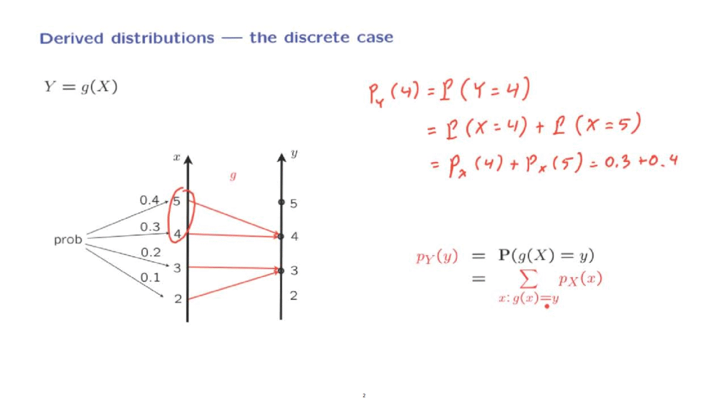
So the probability that the random variable capital Y, which is the same as g of X, takes on a specific value is the sum of the probabilities of all possible values of little x where we only consider those values of little x that give rise to the specific value, little y, that you’re interested.
Let us now look into the special case where we have a linear function of a discrete random variable.
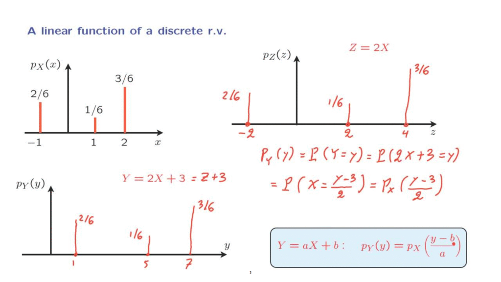
Suppose that X is described by the PMF shown in this diagram, and let us consider the random variable Z, which is defined as 2 times X.
We would like to plot the PMF of Z.
First, let us note the values that Z can take.
When X is equal to minus 1, Z is going to be equal to minus 2.
When X is equal to 1, Z is going to be equal to 2.
And when X is equal to 2, Z is going to be equal to 4.
This event that X is equal to minus 1 happens with probability 2/6, and when that event happens, Z will take a value of minus 2.
So this event happens with probability 2/6.
With probability 1/6, X takes a value of 1 so that Z takes a value of 2.
And this happens with probability 1/6.
6 And finally, this last event here happens with probability 3/6.
We have thus found the PMF of Z.
Notice that it has the same shape as the PMF of X, except that it is stretched or scaled horizontally by a factor of 2.
Let us now consider the random variable Y, defined as 2X plus 3, or what is the same as Z plus 3.
With probability 2/6, Z is equal to minus 2.
And in that case, Y is going to be equal to plus 1.
And this event happens with probability 2/6.
With probability 1/6, Z takes a value of 2 so that Y it takes a value of 5.
And finally, with probability 3/6, Z takes a value of 4 so that Y it takes a value of 7.
What we see here is that the PMF of Y has exactly the same shape as the PMF of Z, except that it is shifted to the right by 3.
To summarize, in order to find the PMF of a linear function such as 2X plus 3, what we do is that we first stretch the PMF of X by a factor of 2 and then shift it horizontally by 3.
We can also describe the PMF of Y through a formula.
For any given value of little y, the PMF is going to be equal to the probability that our random variable Y takes on the specific value little y.
Then we recall that Y has been defined in our example to be equal to 2X plus 3, so we’re looking at the probability of this event.
But this is the same as the event that X takes a value equal to y minus 3 divided by 2.
And in PMF notation, we can write it in this form.
So what this is saying is that the probability that Y takes on a specific value is the same as the probability that X takes on some other specific value.
And that value here is that value of X that would give rise to this particular value little y.
Now, we can generalize the calculation that we just did.
And more generally, if we have a linear function of a discrete random variable X, the PMF of the random variable Y is given by this formula in terms of the PMF of the random variable X.
The derivation is the same.
We use b instead the specific number 3, and we have a general constant a instead of the 2 that we had in this example.
And this formula describes exactly what we did graphically in our previous example.
This factor of a here serves to stretch the PMF by a factor of a, and this term b here serves to shift the PMF by b.