We have seen that several properties, such as, for example, linearity of expectations, are common for discrete and continuous random variables.
For this reason, it would be nice to have a way of talking about the distribution of all kinds of random variables without having to keep making a distinction between the different types– discrete or continuous.
This leads us to describe the distribution of a random variable in a new way, in terms of a so-called cumulative distribution function or CDF for short.
A CDF is defined as follows.
The CDF is a function of a single argument, which we denote by little x in this case.
And it gives us the probability that the random variable takes a value less than or equal to this particular little x.
We will always use uppercase Fs to indicate CDFs.
And we will always have some subscripts that indicate which random variable we’re talking about.
The beauty of the CDF is that it just involves a probability– a concept that is well defined, no matter what kind of random variable we’re dealing with.
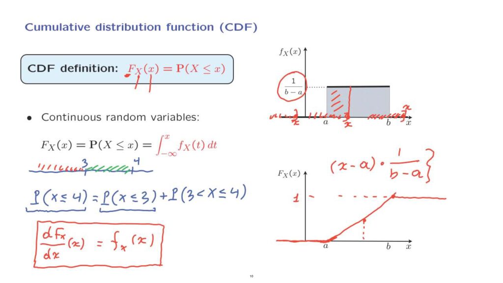
So in particular, if X is a continuous random variable, the probability that X is less than or equal to a certain number– this is just the integral of the PDF over that range from minus infinity up to that number.
As a more concrete example, let us consider a uniform random variable that ranges between a and b, and let us just try to plot the corresponding CDF.
The CDF is a function of little x.
And the form that it takes depends on what kind of x we’re talking about.
If little x falls somewhere here to the left of a, and we ask for the probability that our random variable takes values in this interval, then this probability will be 0 because all of the probability of this uniform is between a and b.
Therefore, the CDF is going to be 0 for values of x less than or equal to a.
How about the case where x lies somewhere between a and b? In that case, the probability that our random variable falls to the left of here– this is whatever mass there is under the PDF when we consider the integral up to this particular point.
So we’re looking at the area under the PDF up to this particular point x.
This area is of the form the base of the rectangle, which is x minus a, times the height of the rectangle, which is 1 over b minus a.
This is a linear function in x that takes the value of 0 when x is equal to a, grows linearly, and when x reaches a value of b, it becomes equal to 1.
How about the case where x lies to the right of b? We’re talking about the probability that our random variable takes values less than or equal to this particular x.
But this includes the entire probability mass of this uniform.
We have unit mass on this particular interval, so the probability of falling to the left of here is equal to 1.
And this is the shape of the CDF for the case of a uniform random variable.
It starts at 0, eventually it rises, and eventually it reaches a value of 1 and stays constant.
Coming back to the general case, CDFs are very useful, because once we know the CDF of a random variable, we have enough information to calculate anything we might want to calculate.
For example, consider the following calculation.
Let us look at the range of numbers from minus infinity to 3 and then up to 4.
If we want to calculate the probability that X is less than or equal to 4, we can break it down as the probability that X is less than or equal to 3– this is one term– plus the probability that X falls between 3 and 4, which would be this event here.
So this equality is true because of the additivity property of probabilities.
This event is broken down into two possible events.
Either x is less than or equal to 3 or x is bigger than 3 but less than or equal to 4.
But now we recognize that if we know the CDF of the random variable, then we know this quantity.
We also know this quantity, and this allows us to calculate this quantity.
So we can calculate the probability of a more general interval.
So in general, the CDF contains all available probabilistic information about a random variable.
It is just a different way of describing the probability distribution.
From the CDF, we can recover any quantity we might wish to know.
And for continuous random variables, the CDF actually has enough information for us to be able to recover the PDF.
How can we do that? Let’s look at this relation here, and let’s take derivatives of both sides.
On the left, we obtain the derivative of the CDF.
And let’s evaluate it at a particular point x.
What do we get on the right? By basic calculus results, the derivative of an integral, with respect to the upper limit of the integration, is just the integrand itself.
So it is the density itself.
So this is a very useful formula, which tells us that once we have the CDF, we can calculate the PDF.
And conversely, if we have the PDF, we can find the CDF by integrating.
Of course, this formula can only be correct at those places where the CDF has a derivative.
For example, at this corner here, the derivative of the CDF is not well defined.
We would get a different value if we differentiate from the left, a different value when we differentiate from the right, so we cannot apply this formula.
But at those places where the CDF is differentiable, at those places we can find the corresponding value of the PDF.
For instance, in this diagram, at this point the CDF is differentiable.
The derivative is equal to the slope, which is this quantity.
And this quantity happens to be exactly the same as the value of the PDF.
So indeed, here, we see that the PDF can be found by taking the derivative of the CDF.
Now, as we discussed earlier, CDFs are relevant to all types of random variables.
So in particular, they are also relevant to discrete random variables.
For a discrete random variable, the CDF is, of course, defined the same way, except that we calculate this probability by adding the probabilities of all possible values of the random variable that are less than [or equal to] the particular little x that we’re considering.
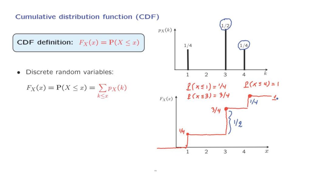
So we have a summation instead of an integral.
Let us look at an example.
This is an example of a discrete random variable described by a PMF.
And let us try to calculate the corresponding CDF.
The probability of falling to the left of this number, for example, is equal to 0.
And all the way up to 1, there is 0 probability of getting a value for the random variable less than that.
But now, if we let x to be equal to 1, then we’re talking about the probability that the random variable takes a value less than or equal to 1.
And because this includes the value of 1, this probability would be equal to 1/4.
This means that once we reach this point, the value of the CDF becomes 1/4.
At this point, the CDF makes a jump.
At 1, the value of the CDF is equal to 1/4.
Just before 1, the value of the CDF was equal to 0.
Now what’s the probability of falling to the left of, let’s say, 2? This probability is again 1/4.
There’s no change in the probability as we keep moving inside this interval.
So the CDF stays constant, until at some point we reach the value of 3.
And at that point, the probability that the random variable takes a value less than or equal to 3 is going to be the probability of a 3 plus the probability of a 1 which becomes 3 over 4.
For any other x in this interval, the probability that the random variable takes a value less than this number will stay at 1/4 plus 1/2, so the CDF stays constant.
And at this point, the probability of being less than or equal to 4, this probability becomes 1.
And so the CDF jumps once more to a value of 1.
Again, at the places where the CDF makes a jump, which one of the two is the correct value? The correct value is this one.
And this is because the CDF is defined by using a less than or equal sign in the probability involved here.
So in the case of discrete random variables, the CDF takes the form of a staircase function.
It starts at 0.
It ends up at 1.
It has a jump at those points where the PMF assigns a positive mass.
And the size of the jump is exactly equal to the corresponding value of the PMF.
Similarly, the size of the PMF here is 1/4, and so the size of the corresponding jump at the CDF will also be equal to 1/4.
CDFs have some general properties, and we have seen a hint of those properties in what we have done so far.
So the CDF is, by definition, the probability of obtaining a value less than or equal to a certain number little x.
It’s the probability of this interval.
If I were to take a larger interval, and go up to some larger number y, this would be the probability of a bigger interval.
So that probability would only be bigger.
And this translates into the fact that the CDF is an non-decreasing function.
If y is larger than or equal to x, as in this picture, then the value of the CDF evaluated at that point y is going to be larger than or equal to the CDF evaluated at that point little x.
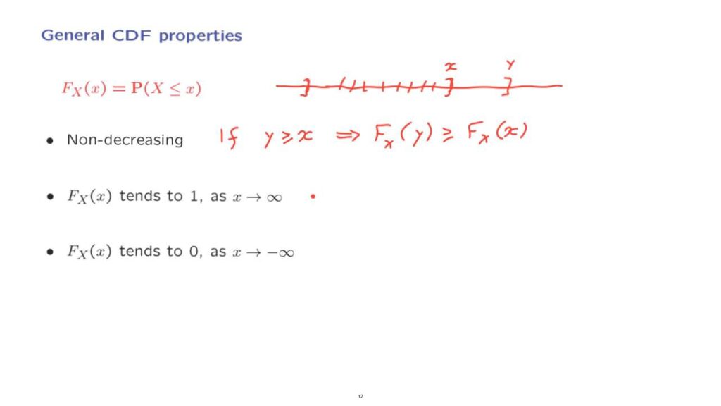
Other properties that the CDF has is that as x goes to infinity, we’re talking about the probability essentially of the entire real line.
And so the CDF will converge to 1.
On the other hand, if x tends to minus infinity, so we’re talking about the probability of an interval to the left of a point that’s all the way out, further and further out.
That probability has to diminish, and eventually converge to 0.
So in general, CDFs asymptotically start at 0.
They can never go down.
They can only go up.
And in the limit, as x goes to infinity, the CDF has to approach 1.
Actually in the examples that we saw earlier, it reaches the value of 1 after a certain finite point.
But in general, for general random variables, it might only reach the value 1 asymptotically.