We have introduced the concept of expected value or mean, which tells us the average value of a random variable.
We will now introduce another quantity, the variance, which quantifies the spread of the distribution of a random variable.
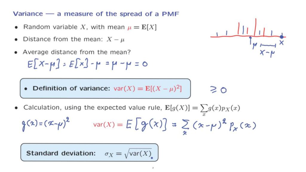
So consider a random variable with a given PMF, for example like the PMF shown in this diagram.
And consider another random variable that happens to have the same mean, but it’s distribution is more spread out.
So both random variables have the same mean, which we denote by mu, and which in this picture would be somewhere around here.
However, the second PMF, the blue PMF, has typical outcomes that tend to have a larger distance from the mean.
By distance from the mean what we mean is that if the result of the random variable, its numerical value, happens to be, let’s say for example, this one, then this quantity here is X minus mu is the distance from the mean, how far away the outcome of the random variable happens to be from the mean of that random variable.
Of course, the distance from the mean is a random quantity.
It is a random variable.
Its value is determined once we know the outcome of the experiment and the value of the random variable.
What can we say about the distance from the mean.
Let us calculate its average or expected value.
The expected value of the distance from the mean, which is this quantity, using the linearity of expectations, is equal to the expected value of X minus the constant mu.
But the expected value is by definition equal to mu.
And so we obtain zero.
So we see that the average value of the distance from the mean is always zero.
And so it is uninformative.
What we really want is the average absolute value of the distance from the mean, or something with this flavor.
Mathematically, it turns out that the average of the squared distance from the mean is a better behaved mathematical object.
And this is the quantity that we will consider.
It has a name.
It is called the variance.
And it is defined as the expected value of the squared distance from the mean.
The first thing to note is that the variance is always non-negative.
This is because it is the expected value of non-negative quantities.
How exactly do we computer the variance? The squared distance from the mean is really a function of the random variable X.
So it is a function of the form g of X, where g is a particular function defined this way.
So we can use the expected value rule applied to this particular function g.
And we obtain the following.
So what we have to do is to go over all numerical values of the random variable X.
For each one, calculate its squared distance from the mean and weigh that quantity according to the corresponding probability of that particular numerical value.
One final comment, the variance is a bit hard to interpret, because it is in the wrong units.
If capital X corresponds to meters, then the variance has units of meters squared.
A more intuitive quantity is the square root of the variance, which is called the standard deviation.
It has the same units as the random variable and captures the width of the distribution.
Let us now take a quick look at some of the properties of the variance.
We know that expectations have a linearity property.
Is this the case for the variance as well? Not quite.
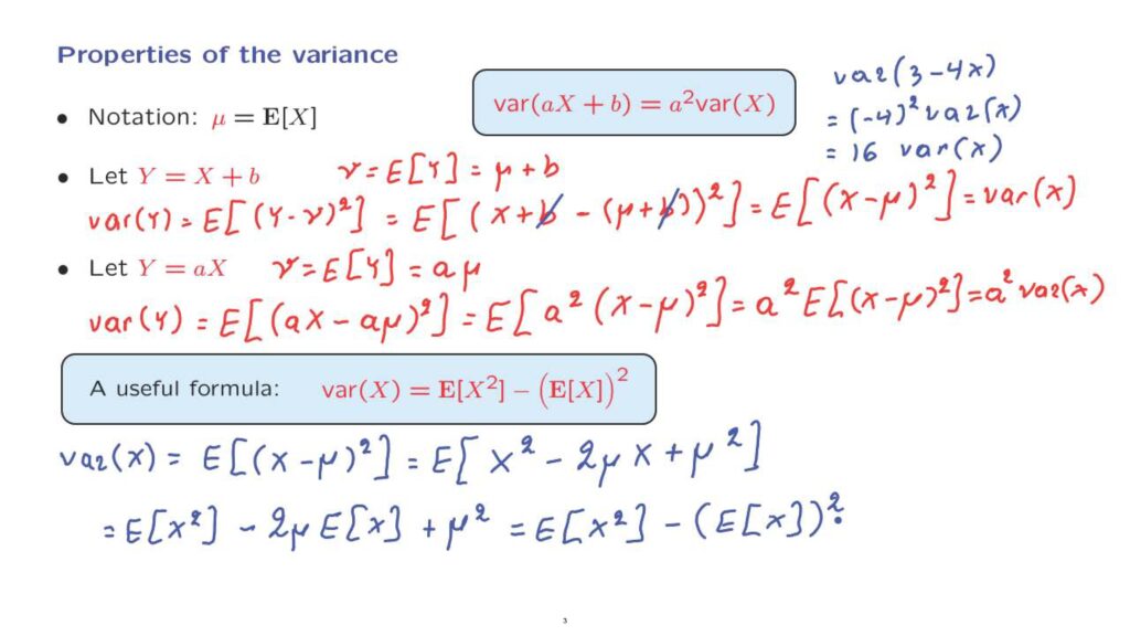
Instead we have this relation for the variance of a linear function of a random variable.
Let us see why it is true.
We use the shorthand notation mu for the expected value of X.
We will proceed one step at a time and first consider what happens to the variance if we add the constant to a random variable.
So let Y be X plus some constant b.
And let us just define nu to be the expected value of Y, which, using linearity of expectations, is the expected value of X plus b.
Let us now calculate the variance.
By definition the variance of Y is the expected value of the distance squared of Y from its mean.
Now we substitute, because in this case Y is equal to X plus b.
Whereas the mean, nu, is mu plus b.
And now we notice that this b cancels with that b.
And we are left with the expected value of X minus mu squared, which is just the variance of X.
So this proves this relation for the case where a is equal to 1.
The variance of X plus b is equal to the variance of X.
So we see that when we add a constant to a random variable, the variance remains unchanged.
Intuitively, adding a constant just moves the entire PMF right or left by some amount, but without changing its shape.
And so the spread of this PMF remains unchanged.
Let us now see what happens if we multiply a random variable by a constant.
Let again nu be the expected value of Y.
And so in this case by linearity this is equal to a times the expected value of X.
So it is a times mu.
We calculate the variance once more using the definition and substituting in the place of Y what Y is in this case– it’s aX– and subtracting the mean of Y, which is a mu, squared.
We take out a factor of a squared.
And then we use linearity of expectations to note that this is a squared times the expected value of X minus mu squared, which is a squared times the variance of X.
So this establishes this formula for the case where b equals zero.
Putting together these two facts, if we multiply a random variable by a, the variance gets multiplied by a squared.
And if we add a constant, the variance doesn’t change.
And this establishes this particular fact.
As an example, the variance of, let’s say, 3 minus 4X is going to be equal minus 4 squared times the variance of X, which is 16 times the variance of X.
Finally, let me mention an alternative way of computing variances, which is often a bit quicker.
We have this useful formula here.
We will see later a few examples of how it is used, but for now let me just show why it is true.
We have by definition that the variance of X is the expected value of X minus mu squared.
Now let us rewrite what is inside the expectation by just expanding this square, which is [X squared minus] 2 mu X plus mu squared.
Using linearity of expectations, this is broken down into expected value of X squared minus the expected value of two times mu X.
But mu is a constant.
So we can take it outside the expected value.
And we’re left with 2mu expected value of X plus mu squared.
But remember that mu is just the same as the expected value of X.
So what we have here is twice the expected value of X, squared, plus the expected value of X, squared, and that leaves us just minus the expected value of X, squared.
So we will now move in the next segment into a few examples of variance calculations.