The next random variable that we will discuss is the binomial random variable.
It is one that is already familiar to us in most respects.
It is associated with the experiment of taking a coin and tossing it n times independently.
And at each toss, there is a probability, p, of obtaining heads.
So the experiment is completely specified in terms of two parameters– n, the number of tosses, and p, the probability of heads at each one of the tosses.
We can represent this experiment by the usual sequential tree diagram.
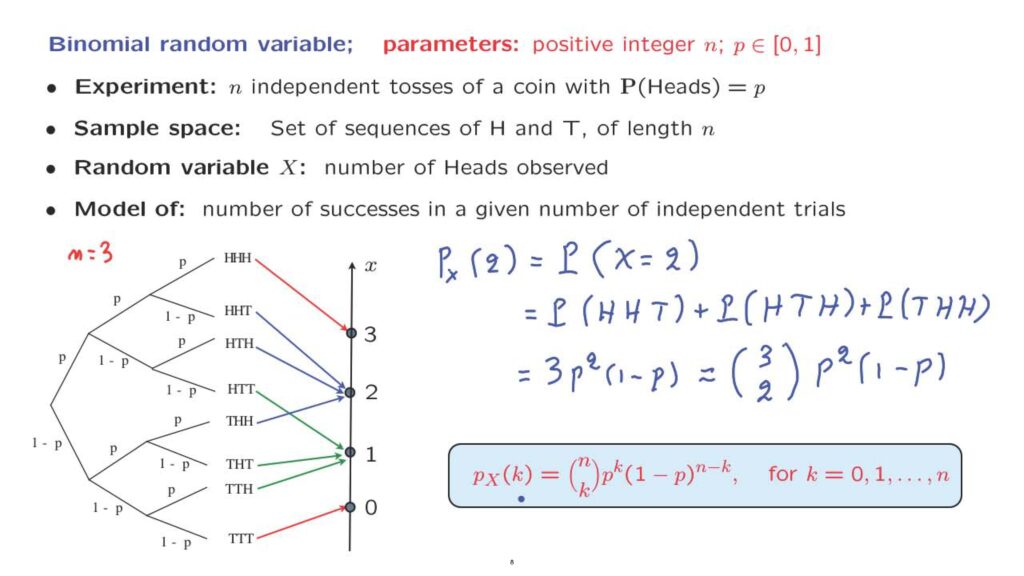
And the leaves of the tree are the possible outcomes of the experiment.
So these are the elements of the sample space.
And a typical outcome is a particular sequence of heads and tails that has length n.
In this diagram here, we took n to be equal to 3.
We can now define a random variable associated with this experiment.
Our random variable that we denote by capital X is the number of heads that are observed.
So for example, if the outcome happens to be this one– tails, heads, heads– we have 2 heads that are observed.
And the numerical value of our random variable is equal to 2.
In general, this random variable, a binomial random variable, can be used to model any kind of situation in which we have a fixed number of independent trials and identical trials, and each trial can result in success or failure, and we have a probability of success equal to some given number, p.
The number of successes obtained in these trials is, of course, random and it is modeled by a binomial random variable.
We can now proceed and calculate the PMF of this random variable.
Instead of calculating the whole PMF, let us look at just one typical entry of the PMF.
Let’s look at this entry, which, by definition, is the probability that our random variable takes the value of 2.
Now, the random variable taking the numerical value of 2, this is an event that can happen in three possible ways that we can identify in the sample space.
We can have 2 heads followed by a tail.
We can have heads, tails, heads.
Or we can have tails, heads, heads.
The probability of this outcome is p times p times (1 minus p).
So it’s p squared times (1 minus p).
And the other two outcomes also have the same probability, so the overall probability is 3 times this.
Which can also be written this way, 3 is the same as 3-choose-2.
It’s the number of ways that you can choose 2 heads, where they will be placed in a sequence of 3 slots or 3 trials.
More generally, we have the familiar binomial formula.
So this is a formula that you have already seen.
It’s the probability of obtaining k successes in a sequence of n independent trials.
The only thing that is new is that instead of using the traditional probability notation, now we’re using PMF notation.
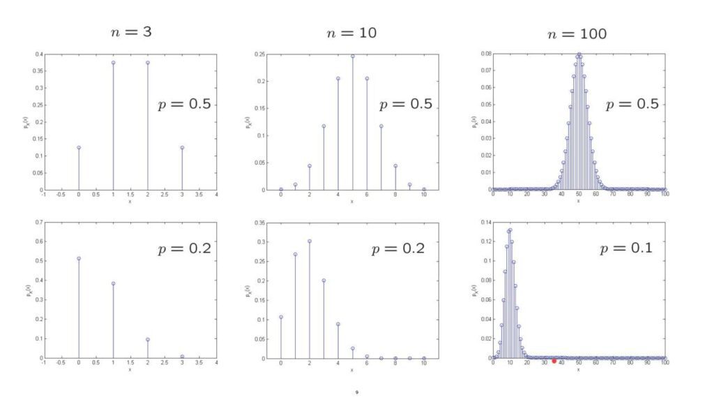
To get a feel for the binomial PMF, it’s instructive to look at some plots.
So suppose that we toss the coin three times and that the coin tosses are fair, so that the probability of heads is equal to 1/2.
Then we see that 1 head or 2 heads are equally likely, and they are more likely than the outcome of 0 or 3 heads.
Now, if we change the number of tosses and toss the coin 10 times, then we see that the most likely result is to have 5 heads.
And then as we move away from 5 in either direction, the probability of that particular result becomes smaller and smaller.
Now, if we toss the coin many times, let’s say 100 times, the coin is still fair, then we see that the number of heads that we’re going to get is most likely to be somewhere in this range between, let’s say, 35 and 65.
These are values of the random variable that have some noticeable or high probabilities.
But anything below 30 or anything about 70 is extremely unlikely to occur.
We can generate similar plots for unfair coins.
So suppose now that our coin is biased and the probability of heads is quite low, equal to 0.2.
In that case, the most likely result is that we’re going to see 0 heads.
And then, there’s smaller and smaller probability of obtaining more heads.
On the other hand, if we toss the coin 10 times, we expect to see a few heads, not a very large number, but some number of heads between, let’s say, 0 and 4.
Finally, if we toss the coin 100 times and we take the coin to be an extremely unfair one, what do we expect to see?
If we think of probabilities as frequencies, we expect to see heads roughly 10% of the time.
So, given that n is 100, we expect to see about 10 heads. But when we say about 10 heads, we do not mean exactly 10 heads.
About 10 heads, in this instance, as this plot tells us, is any number more or less in the range from 0 to 20. But anything above 20 is extremely unlikely.