In this segment, we discuss the expected value rule for calculating the expected value of a function of a random variable.
It corresponds to a nice formula that we will see shortly, but it also involves a much more general idea that we will encounter many times in this course, in somewhat different forms.
Here’s what it is all about.
We start with a certain random variable that has a known PMF.
However, we’re ultimately interested in another random variable Y, which is defined as a function of the original random variable.
We’re interested in calculating the expected value of this new random variable, Y.
How should we do it? We will illustrate the ideas involved through a simple numerical example.
In this example, we have a random variable, X, that takes values 2, 3, 4, or 5, according to some given probabilities.
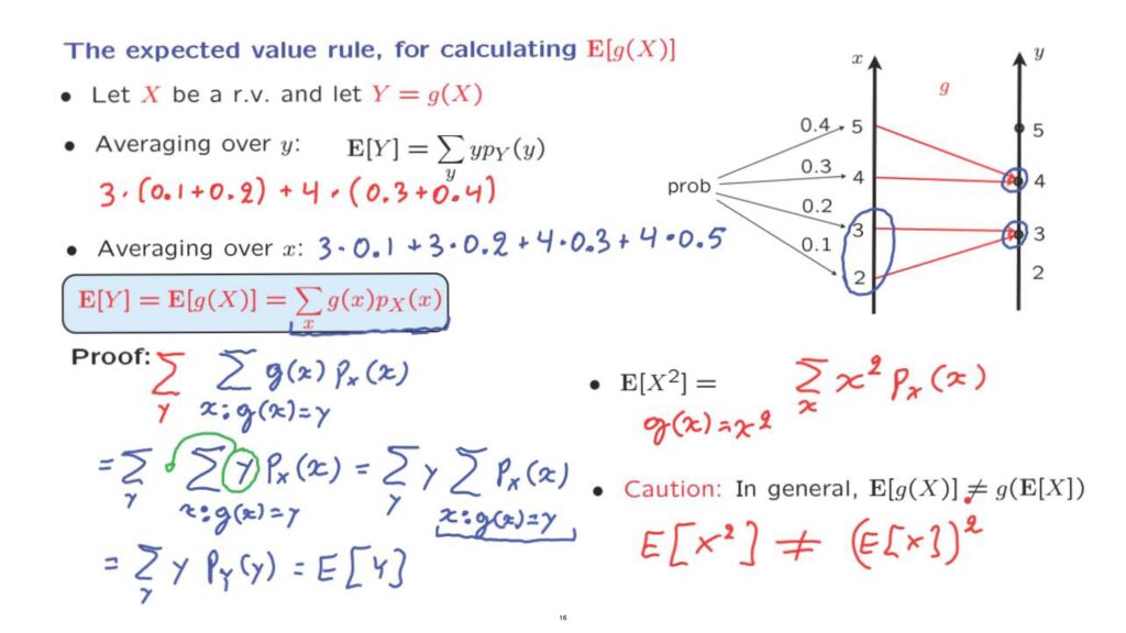
We are also given a function that maps x-values into y-values.
And this function, g, then defines a new random variable.
So if the outcome of the experiment leads to an X equal to 4, then the random variable, Y, will also take a value equal to 4.
How do we calculate the expected value of Y? The only tool that we have available in our hands at this point is the definition of the expected value, which tells us that we should run a summation over the y-axis, consider different values of y one at the time.
And for each value for y, multiply that value by its corresponding probability.
So in this case, we start with Y equal to 3, which needs to be multiplied by the probability that Y is equal to 3.
What is that probability? Well, Y is equal to three, if and only if X is 2 or 3, which happens with probability, 0.1 plus 0.2.
Then we continue with the summation by considering the next value of little y.
The next possible value is 4.
And this gives us a contribution of 4, weighted by the probability of obtaining a 4.
The probability that Y is equal to 4 is the probability that X is either equal to 4 or to 5, which happens with probability.
0.3 plus 0.4.
So this way, we obtain an arithmetic expression which we can evaluate.
And it’s going to give us the expected value of Y.
But here’s an alternative way of calculating the expected value.
And this corresponds to the following type of thinking.
10% of the time, X is going to be equal to 2.
And when that happens, Y takes on a value of 3.
So this should give us a contribution to the average value of Y, which is 3 times 0.1.
Then, 20% of the time, X is 3 and Y is also 3.
So 20% of the time, we also get 3’s in Y.
Then 30% of the time, X is 4, which results in a Y that’s equal to 4.
So we obtain a 4 30% of the time.
And finally, 40% of the time, X equals to [5], which results in a Y equal to 4.
And we obtain this arithmetic expression.
Now you can compare the two arithmetic expressions, the red and the blue one, and you will notice that they’re equal, except that the terms are arranged in a slightly different way.
Conceptually, however, there’s a very big difference.
In the first summation, we run over the values of Y one at the time.
In the second summation, we run over the different values of X one at a time, and took into account their individual contributions.
This second way of calculating the expected value of Y is called the expected value rule.
And it corresponds to the following formula.
We carry out a summation over the x-axis.
For each x-value that we consider, we calculate what is the corresponding y-value, that’s g of x, and also weigh this term according to the probability of this particular x.
So for instance, a typical term here would be when x is equal to 2, g of x would be equal to 3.
And the corresponding probability, that’s the probability of a 2, would be 0.1.
The advantage of using the expected value rule instead of the definition of the expectation is that the expected value rule only involves the PMF of the original random variable, so we do not need to do any additional work to find the PMF of the new random variable.
Now we argued in favor of the expected value rule by considering this numerical example, and by checking that it gives the right result.
But now let us verify.
Let us argue more generally that it’s going to give us the right answer.
So what we’re going to do is to take this summation and argue that it’s equal to the expected value of Y, which is defined by that summation.
So let us start with this.
It’s a sum over all x’s.
Let us first fix a particular value of y, and add over all those x’s that correspond to that particular y.
So we’re fixing a particular y.
And so we’re adding only over those x’s that lead to that particular y.
And we carry out to the summation.
So this is the part of this sum associated with one particular choice of y.
And it’s a sum, really, over this set of x’s.
But in order to exhaust all x’s, we need to consider all possible values of y.
And this gives rise to an outer summation over the different y’s.
So for any fixed y, we add over the associated x’s.
But we want to consider all the possible y’s.
Now at this point, we make the following observation.
Here, we have a summation over y’s.
And let’s look at the inner summation.
The inner summation involves x’s, all of which are associated with a specific value of y.
Having fixed y, all the terms inside this sum have the property that g of x is equal to y.
So g of x is equal to that particular y.
And we can make this substitution here.
Now when we look at this summation, we now realize that it’s a summation over x’s while y is being fixed.
And so we can take this term of y and pull it outside the summation.
What this leaves us with is a sum over all y’s of y, and then a further sum over all x’s that lead to that particular y, of the probabilities of those x’s.
Now what can we say about this inner summation? We have fixed a y.
For that particular y, we’re adding the probabilities of all the x’s that lead to that particular y.
Fixing y, consider all the x’s that lead to it.
This is just the probability of that particular y.
But what we have now is just the definition of the expected value of Y.
And this concludes the proof that this expression, as given by the expected value rule, gives us the same answer as the original definition of the expected value of Y.
Now before closing, a few observations.
The expected value rule is really simple to use.
For example, if you want to calculate the expected value of the square of a random variable, then you’re dealing with a situation where the g function is the square function.
And so, the expected value of X-squared will be the sum over x’s of x squared weighted according to the probability of a particular x.
And finally, one important word of caution, that in general, the expected value of the function– so for example, the expected value of X-squared.
In general, it’s not going to be the same as taking the expected value of X and squaring it.
So this is a word [of] caution, that in general, you cannot interchange the order with which you apply a function, and then you calculate expectation.
There are exceptions, however, in which we happen to have equality here.
And this is going to be our next topic.