We have so far discussed the first step involved in the construction of a probabilistic model. Namely, the construction of a sample space, which is a description of the possible outcomes of a probabilistic experiment.
We now come to the second and much more interesting part. We need to specify which outcomes are more likely to occur and which ones are less likely to occur and so on. And we will do that by assigning probabilities to the different outcomes. However, as we try to do this assignment, we run into some kind of difficulty, which is the following.
Remember the previous experiment involving a continuous sample space, which was the unit square and in which we throw a dart at random and record the point that occurred. In this experiment, what do you think is the probability of a particular point? Let’s say what is the probability that my dart hits exactly the center of this square. Well, this probability would be essentially 0.
Hitting the center exactly with infinite precision should be 0. And so it’s natural that in such a continuous model any individual point should have a 0 probability. For this reason instead of assigning probabilities to individual points, we will instead assign probabilities to whole sets, that is, to subsets of the sample space. So here we have our sample space, which is some abstract set omega.
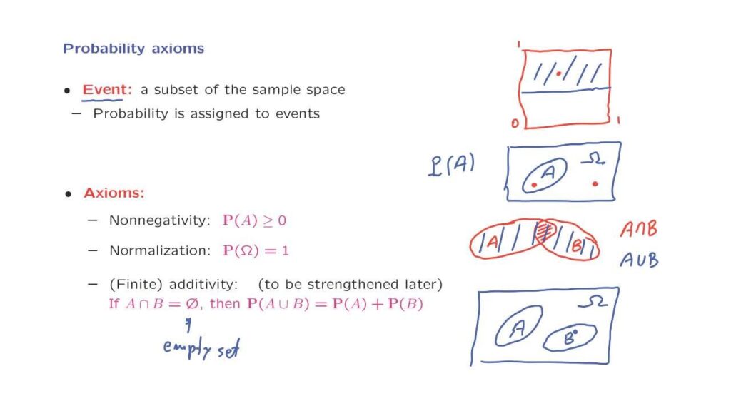
Here is a subset of the sample space. Call it capital A. We’re going to assign a probability to that subset A, which we’re going to denote with this notation, which we read as the probability of set A. So probabilities will be assigned to subsets.
And these will not cause us difficulties in the continuous case because even though individual points would have 0 probability, if you ask me what are the odds that my dart falls in the upper half, let’s say, of this diagram, then that should be a reasonable positive number.
So even though individual outcomes may have 0 probabilities, sets of outcomes in general would be expected to have positive probabilities. So coming back, we’re going to assign probabilities to the various subsets of the sample space. And here comes a piece of terminology, that a subset of the sample space is called an event.
Why is it called an event? Because once we carry out the experiment and we observe the outcome of the experiment, either this outcome is inside the set A and in that case we say that event A has occurred, or the outcome falls outside the set A in which case we say that event A did not occur.
Now we want to move on and describe certain rules. The rules of the game in probabilistic models, which are basically the rules that these probabilities should satisfy. They shouldn’t be completely arbitrary.
First, by convention, probabilities are always given in the range between 0 and 1. Intuitively, 0 probability means that we believe that something practically cannot happen. And probability of 1 means that we’re practically certain that an event of interest is going to happen.
So we want to specify rules of these kind for probabilities. These rules that any probabilistic model should satisfy are called the axioms of probability theory.
And our first axiom is a nonnegativity axiom. Namely, probabilities will always be non-negative numbers. It’s a reasonable rule.
The second rule is that if the subset that we’re looking at is actually not a subset but is the entire sample space omega, the probability of it should always be equal to 1. What does that mean? We know that the outcome is going to be an element of the sample space.
This is the definition of the sample space.
So we have absolute certainty that our outcome is going to be in omega. Or in different language we have absolute certainty that event omega is going to occur. And we capture this certainty by saying that the probability of event omega is equal to 1.
These two axioms are pretty simple and very intuitive. The more interesting axiom is the next one that says something a little more complicated. Before we discuss that particular axiom, a quick reminder about set theoretic notation.
If we have two sets, let’s say a set A, and another set, another set B, we use this particular notation, which we read as “A intersection B” to refer to the collection of elements that belong to both A and B. So in this picture, the intersection of A and B is this shaded set.
We use this notation, which we read as “A union B”, to refer to the set of elements that belong to A or to B or to both. So in terms of this picture, the union of the two sets would be this blue set.
After this reminder about set theoretic notation, now let us look at the form of the third axiom. What does it say? If we have two sets, two events, two subsets of the sample space, which are disjoint.
So here’s our sample space. And here are the two sets that are disjoint. In mathematical terms, two sets being disjoint means that their intersection has no elements. So their intersection is the empty set.
And we use this symbol here to denote the empty set. So if the intersection of two sets is empty, then the probability that the outcome of the experiments falls in the union of A and B, that is, the probability that the outcome is here or there, is equal to the sum of the probabilities of these two sets. This is called the additivity axiom.
So it says that we can add probabilities of different sets when those two sets are disjoint. In some sense we can think of probability as being one pound of some substance which is spread over our sample space and the probability of A is how much of that substance is sitting on top of a set A.
So what this axiom is saying is that the total amount of that substance sitting on top of A and B is how much is sitting on top of A plus how much is sitting on top of B. And that is the case whenever the sets A and B are disjoint from each other.
The additivity axiom needs to be refined a bit. We will talk about that a little later. Other than this refinement, these three axioms are the only requirements in order to have a legitimate probability model. At this point you may ask, shouldn’t there be more requirements?
Shouldn’t we, for example, say that probabilities cannot be greater than 1?
Yes and no. We do not want probabilities to be larger than 1, but we do not need to say it. As we will see in the next segment, such a requirement follows from what we have already said.
And the same is true for several other natural properties of probabilities.