Let us now come back to the trajectory estimation problem that we introduced earlier.
We have an object that moves vertically.
At any given time t, the height at which the object is found is equal to this expression.
It corresponds to the following– the object starts at time 0, at some initial height Theta0, it has an initial velocity of Theta1, but also has a certain acceleration.
And if Theta2 is negative, this will be a downwards acceleration, which means that the object eventually will turn and start going down.
So this is a typical trajectory of such an object, where here we’re plotting the height as a function of time.
However, the Thetas are unknown and they are random– we do not know what they are.
So this blue curve is just a simulation where we drew values for those random variables at random.
But if we were to simulate again, we might obtain a somewhat different blue curve, because the values of the Thetas might have been different.
We do not observe the true trajectory directly.
What we do observe is certain data points.
What are they?
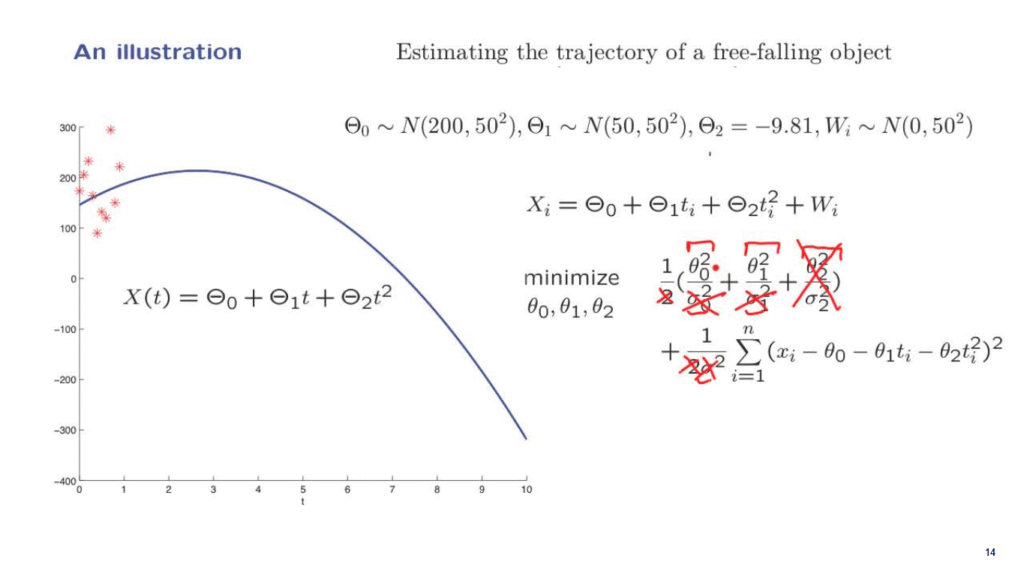
At certain times ti we make a measurement of the height of the object, except that this measurement is corrupted by some additive noise.
This is the model that we introduced earlier.
And our assumptions were that all of the random variables involved– the Thetas and the W’s were normal with 0 mean and were also independent.
In that case, we saw that maximizing the posterior distribution of the Thetas after taking logarithms amounted to minimizing this quadratic function of the thetas.
So once we have some data available in our hands, we look at this expression as a function of the thetas and find the thetas that are as as good as possible in terms of this criterion.
And this is the MAP methodology for this particular example.
Now, for the purposes of this illustration, actually, we will change our assumptions a little bit.
They will be as follows.
Regarding the acceleration, we will take it to be a constant.
The acceleration term often has to do with gravitational effects which are known, so we will treat Theta2 as a constant.
And that means that there’s no point in having a prior distribution for Theta2.
So this term here, which originated from the prior distribution of Theta2 is going to disappear.
We will take the variances of these basic random variables to be the same.
And because of this, these constants here will all be the same.
Therefore, we can take them outside of this expression, and outside the minimization they will not matter.
So we can remove them from the picture.
The factor of 1/2 can also be removed similarly.
It does not affect the minimization.
Finally, just in order to get a nicer illustration, instead of taking 0 means, we’re assuming that the initial position has a mean of 200.
So we’re starting somewhere around here.
And furthermore, the initial velocity has a mean of 50.
So we expect the object to start moving upwards.
How does this change the formulation?
Well, remember, that this term and this term originated from the priors for Theta0 and Theta1.
If we now change the means, the priors will change.
And what happens, if you recall the formula for the normal PDF and how the mean enters, after you take logarithms, you see that instead of having here theta0, you should have theta0 minus the mean of theta0 squared.
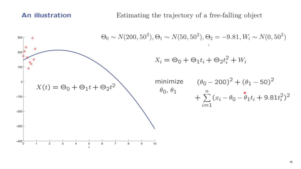
And this leads us to the following formulation.
So this is the formulation that we will consider.
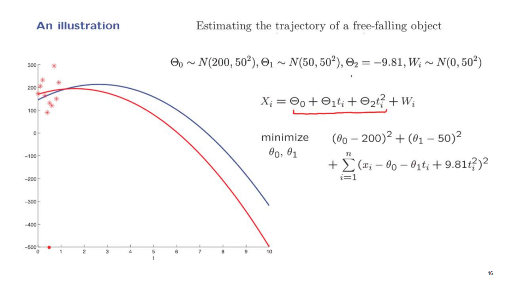
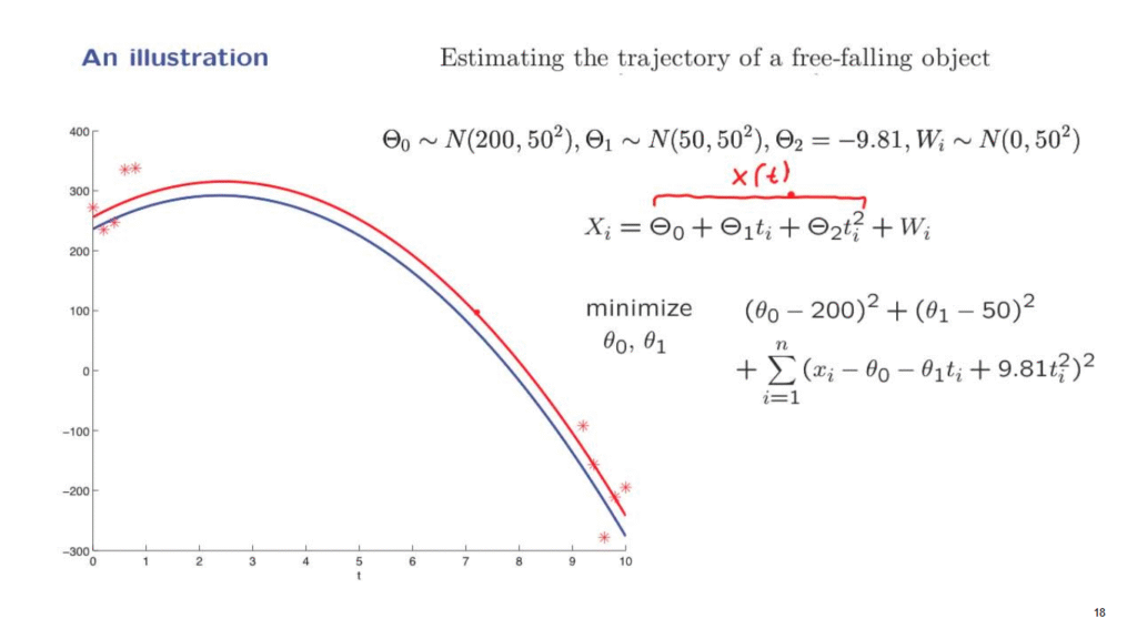
We obtain these data points, and for these particular data points and for known times at which the measurements were taken, we put these numbers into this minimization, carried it out numerically, and this is what we got.
We got estimates for the different parameters.
And using this estimates, we can use this expression to construct an estimated trajectory.
And the estimated trajectory is given by the red curve.
It seems to be doing somewhat of a reasonable job, but not quite.
The distance between these two curves is quite substantial.
How could we do a little better?
Why is it that we’re not doing very well?
Let’s think intuitively.
One of the parameters we wish to estimate is Theta1.
And Theta1 is a velocity.
Now, all of our measurements are concentrated at pretty much the same time.
But if you measure an object only at a certain time, it is very difficult to estimate its velocity.
A much better idea would be to try to measure the position of the object at different times and use that information to estimate velocity.
So let us instead of taking all the measurements around the initial time, have five measurements in the beginning and five measurements towards the end.
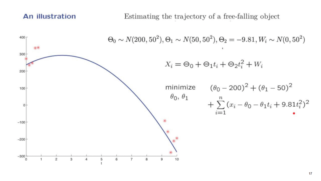
The total number of measurements in this example is the same as in the previous example.
And once more, we generate a simulated trajectory according to the probability distributions that we are assuming.
Then we generate data according to this model and we wish to estimate this trajectory.
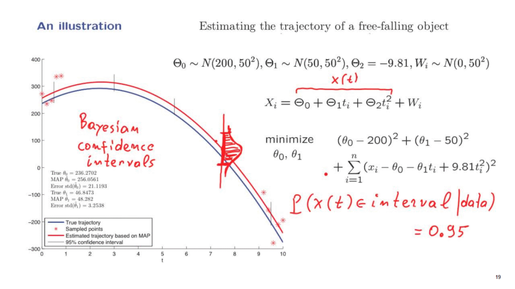
We take the data, plug them into this minimization, carry it out numerically, and this is what we obtain.
So we see that here we are doing a lot better.
The estimated trajectory is quite close to the unknown blue trajectory, even though the data seems to be scattered quite a bit.
This is a very nice property.
But is it just an accident of this numerical experiment?
Or, also, to put it differently, once you get your estimated trajectory, yes, it is true that it is close to the blue trajectory, but you do not necessarily know that fact.
It is one thing to have an estimate that is close to the true value, and it’s a different thing to have an estimate that you know that it is close to the true value.
So how could we get some guarantees that, indeed, this is the case, that we have good estimates?
Here’s how it goes.
As we discussed before, the posterior distribution of the Thetas given the data is normal.
And for similar reasons, the posterior distribution of this quantity, which is the true position, it’s what we denoted by X of t, the posterior distribution of X of t is also normal.
And in fact, what we obtain from this diagram is at any given point it’s the maximum of posteriority probability estimate of the position X of t at that time.
However, besides just this point estimate, we have additional information.
We know that the posterior distribution of X of t is normal.
And so, for example, at this time, this is the peak of the posterior.
This is the maximum a posteriori probability estimate.
By we are also able to calculate the variance of this posterior distribution.
This is a calculation that’s a bit complicated for the multivariate case, for the case where you have multiple unknown parameters.
We will not get into it.
But we did see earlier an example where we had a single unknown parameter, and in which we were able to calculate the variance of the posterior distribution.
So the idea is somewhat similar.
So not only we have an estimate for the position of the object at this particular time, but we also have a probability distribution for what the true position might be.
And once we have such a posterior probability distribution, we can find an interval with the property that 95% of the probability is inside that interval.
In other words, we construct an interval with the property that the probability that X of t belongs to the interval.
(Now, we’re talking about posterior probabilities.
So it is a posterior probability, given the data.
) This probability is, let’s say, 0.
95.
Such an interval gives useful information besides a point estimate, it also gives us a range of possible values.
And outside this range, it is quite unlikely to have the true trajectory be out there.
So here we’re showing some confidence intervals that apply to different times, and they’re pretty narrow, they’re pretty small.
And they indicate, they give us confidence that we have pretty accurate estimates of the true trajectory.
This kind of confidence intervals that we have discussed in the context of this examples are called Bayesian confidence intervals.
And they’re very useful when you report your results, to not just give point estimates, but to also provide confidence intervals.
Coming back to the bigger picture, what happened in this particular example is quite indicative of many real world applications.
One starts with a linear model, in which we have a linear relation between the variables that are unknown and the observations, but where also the observations are corrupted by noise.
One makes certain normality and independence assumptions.
And as long as the modeling has been done carefully and the assumptions are justified, then by carrying out this procedure, one usually obtains estimates that are very helpful and very informative.