In the previous lecture, we went through examples of inference involving some of the variations of the Bayes rule.
One case that we did not consider was the case where the unknown random variable and the observation are both continuous.
In this lecture, we will focus exclusively on an important model of this kind.
And because we consider only one specific setting, we will be able to start it in considerable detail.
In the model that we consider, we start with some basic independent normal random variables.
Some of them, the Theta j, are unknown, to be estimated.
And some of them, the Wi, represent noise.
Our observations, Xi, are linear functions of these basic random variables.
In particular, since linear functions of independent normal random variables are normal, the observations are themselves normal as well.
This is probably the most commonly used type of model in all of inference and statistics.
This is because it is a reasonable approximation in many situations.
Also, it has a very clean analytical structure and a very simple solution.
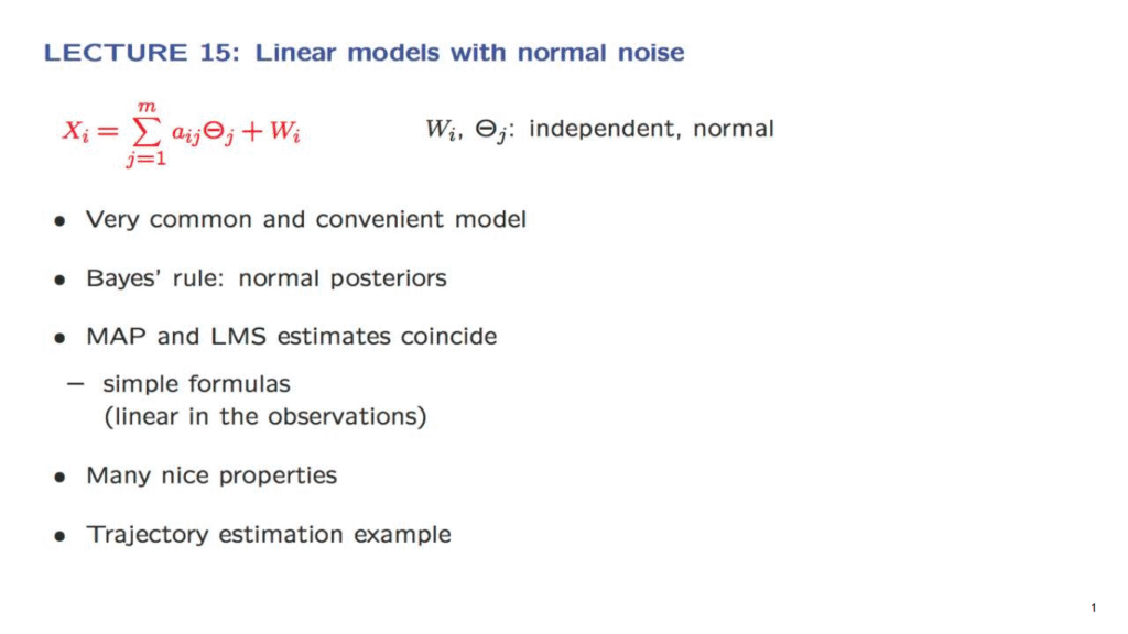
For example, it turns out that the posterior distribution of each Theta j is itself normal and that the MAP and LMS estimates coincide.
This is because the peak of a normal occurs at the mean.
Furthermore, these estimates are given by some simple linear functions of the observations.
We will go over these facts by moving through a sequence of progressively more complex versions.
We will start with just one unknown and one observation and then generalize.
And we will illustrate the formulation and the solution through a rather realistic example where we estimate the trajectory of an object from a few noisy measurements.