In this segment, we make a connection between the correlation coefficient and some fairly realistic real world situations.
The bottom line will be that the presence or absence of correlations can make a huge difference.
Suppose that you run an investment company that invests in real estate, and you have 100 million of capital that you want to invest.
Now you have learned or believe that it helps to diversify, to not put all of your eggs in the same basket.
And for that reason, you’re going to invest some of your money into different states.
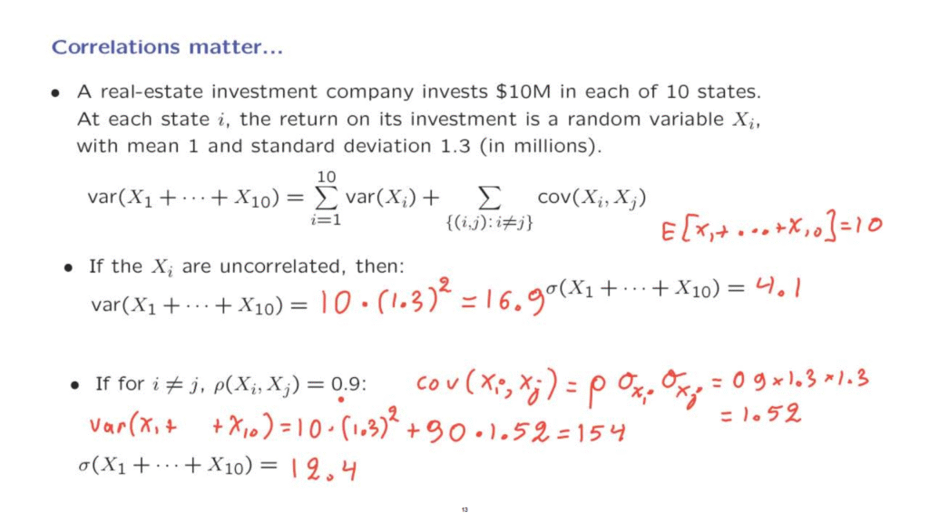
You will be investing in 10 different states, and in each state, you will invest 10 million so that your total investment is spread between those 10 states.
For each state, you have a model that tells you that the return on your investment, that is your profit– It’s, of course, random, but you expect it to be 1 million on the average, that is, in terms of the expected value, but there’s also a fair amount of randomness, and so the standard deviation is 1.3.
Now, if you look at one state in isolation, it would be a pretty risky investment because the standard deviation is comparable to the mean.
It’s not an unlikely event to have a return that’s one standard deviation below the mean.
And if that happens, your return is going to be negative, and you’re losing money.
But then you argue that you’re investing in 10 different states.
Yes, you might lose money in some of them, but overall, you would expect to have a pretty high confidence that you will end up having a positive return.
Is this correct or not?
Let us do some calculations.
We will look at the variance of your total return.
The variance of the sum of random variables is given by the formula that we have developed.
It’s the sum of the variances.
But then you also have a bunch of covariance terms that have to do with the relation of the different random variables.
Now, you make the assumption that the different states are different markets– one doesn’t affect the other– so that the Xi’s are uncorrelated.
In that case, in this variance formula, the covariance terms are all 0, and they disappear and you’re left with the sum of 10 variance terms.
Now, each one of these variances is equal to the square of the standard deviation.
And we have a variance of 16.9.
You then take the square root to find the standard deviation and the square root of this number is 4.1.
Now, your expected return is equal to 10, which is 2 and 1/2 standard deviations.
You will only lose money if the outcome is 2 and 1/2 standard deviations below the mean.
And that’s a fairly unlikely outcome, and so in this situation you feel very confident that you will have a positive profit.
Suppose, however, that your assumption is wrong, and that actually the different Xi’s are correlated with each other.
And suppose that the correlation is pretty high, 0.9.
Essentially, this means that the real estate market in one state is strongly related to the behavior of the market in another state.
And that could be, perhaps, because the markets in different states are affected by some more global phenomenon that operates on a national level.
So in this case, the covariance of Xi with Xj is going to be the correlation coefficient times the standard deviation of Xi times the standard deviation of Xj, which is 0.9 times 1.3 times 1.3.
And so the co-variance turns out to be 1.52.
And in that case, the variance of the sum, using this formula here, is going to be equal to 10 times the variance that you have in each state, which is 1.3 squared, plus you have a bunch of terms here.
How many terms?
There’s 90 of them, and each one of these terms is equal to 1.52.
And the variance turns out to be 154.
Now you take the square root of that, and you find a standard deviation of 12.4.
Now, your expected profit is 10, but the standard deviation is 12.4.
And if you happen to be one standard deviation below the expectation, which is something that has a sizable probability of occurring, then your profit is going to be negative.
So in the uncorrelated case, you’re pretty certain that you will have a positive profit, but if the correlations actually turn out to be significant, then you’re facing a very risky situation.
To some extent, this is similar to what happened during the great financial crisis.
That is, many investment companies thought that they were secure by diversifying and by investing in different housing markets in different states, but then when the economy moved as a whole, it turned out that there were high correlations between the different states, and so the unthinkable, that is large losses, actually did occur.