We work with discrete random variables as a warm up.
And later, we will consider the case of continuous random variables.
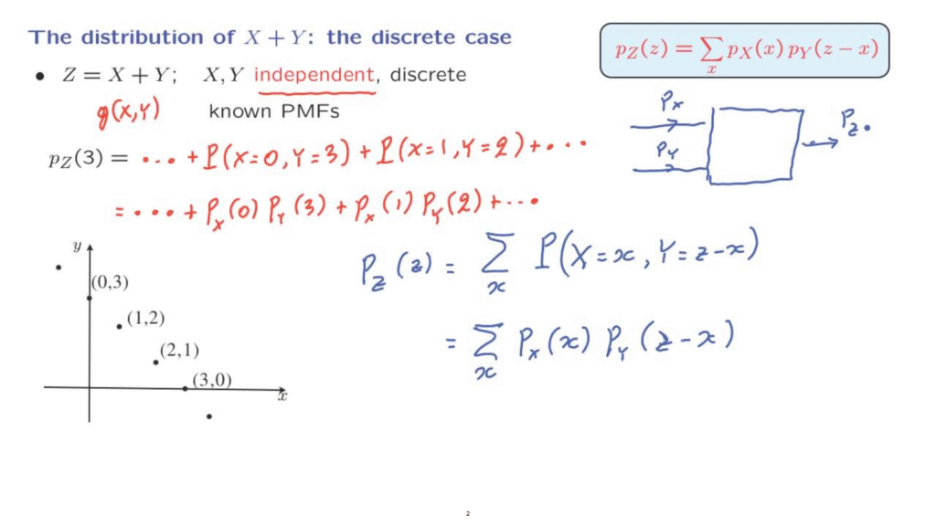
So suppose that we know the PMFs of X and Y and that we want to compute the probability that the sum is equal to 3.
It always helps to have a picture.
The sum of X and Y will be equal to 3.
This is an event that can happen in many ways.
For example, x could be 3 and Y could be 0, or X could be 1 and Y equal to 2.
The probability of the event of interest, that the sum is equal to 3, is going to be the sum of the probabilities of all the different ways that this event can happen.
So it is going to be a sum of various terms.
And the typical term would be the probability, let’s say of this outcome, which is that X is equal to 0 and Y is equal to 3.
Another typical term in the sum will be the probability of this outcome here, the probability that X is equal to 1, Y is equal to 2, and so on.
Now, here comes an important step.
Because we have assumed that X and Y are independent, the probability of these two events happening is the product of the probabilities of each one of these events.
So it is the product of the probability that X is equal to 0, where now I’m using PMF notation, times the probability that Y is equal to 3.
Similarly, the next term is the probability that X is equal to 1 times the probability that Y is equal to 2.
Again, we can do this because we are assuming that our two random variables are independent of each other.
Now, let us generalize.
In the general case, the probability that the sum takes on a particular value little z can be calculated as follows.
We look at all the different ways that the sum of little z can be obtained.
One way is that the random variable X takes on a specific value little X.
And at the same time, the random variable Y takes the value that’s needed so that the sum of the two is equal to little Z.
For a given value of little X, we have a particular way that the sum is equal to Z.
And this particular way has a certain probability.
But little X could be anything.
And different choices of little x give us different ways that the event of interest can happen.
So we add those probabilities over all possible X’s.
And then we proceed as follows.
We invoke independence of X and Y to derive this probability as a product of two probabilities.
And then we use PMF notation instead of probability notation to obtain this expression here.
This formula is called the convolution formula.
It is the convolution of two PMFs.
What convolution means is that somebody gives us the PMF of one random variable, gives us also the PMF of another random variable.
And when we say we’re given the PMF, it means we’re given the values of the PMFs for all the possible choices of little X and little y, the arguments of the two PMFs.
Then the convolution formula does a certain calculation and spits out now a new PMF, which is the PMF of the random variable Z.
Let’s now take a closer look at what it takes to carry out of the calculations involved in this convolution formula.

Let’s proceed by a simple example that will illustrate the methodology.
We’re given two PMFs of two random variables.
And assuming that they are independent, the PMF of their sum is determined by this formula here.
And we want to see what those terms in this summation would be.
Suppose that we’re interested in the probability that the sum is equal to 3.
Now, the sum is going to be equal to 3.
This can happen in several ways.
We could have X equal to 1 and and Y equal to 2.
This combination is one way that the sum of 3 can be obtained.
And that combination has a probability of 1/3 times 3/6.
And that would be one of the terms in this summation.
Another way that the sum of 3 can be obtained is by having X equal to 4 and y equal to minus 1.
And by multiplying this probability 2/3 with 2/6, we obtain another contribution to this summation.
However, keeping track of these correspondences here can become a little complicated if we have richer our PMFs.
So an alternative way of arranging the calculation is the following.
Let us take the PMF of Y, flip it along this vertical axis.
So these two terms would go to the left side, and this term will go to the right hand side.
And then draw it underneath the PMF of X.
This is what we obtain.
Then let us take this drawing here and shift it to the right by 3.
So the entry of minus 2 goes to 1, minus 1 goes to 2, and 1 goes to 4.
So what have we accomplished by these two transformations?
Well, the term that had probability 3/6 and which were to be multiplied with the probability 1/3 on that side, now this 3/6 sits here.
So we have this correspondence.
And we need to multiply 1/3 by 3/6.
Similarly, the multiplication of 2/3 with 2/6 corresponds to the multiplication of this probability here times the probability of this term here.
So when the diagrams are arranged this way, then we have a simpler job to do.
We look at corresponding terms, those that sit on top of each other, multiply them, do that for all the possible choices, and then add those products together.
And this is what we do if we’re shifting by 3.
Now, if we wanted to find the probability that Z equal to 4, we would be doing the same thing, except that this diagram would need to be shifted by one more unit to the right so that we have a total shift of 4.
So we just repeat this procedure for all possible values of Z which corresponds to taking this diagram here and shifting it progressively by different amounts.
This turns out to be a fairly simple and systematic way of arranging the calculations, at least if you’re doing them by hand.
Of course, an alternative is to carry out the calculations on a computer.
This is a pretty simple formula that is not hard to implement on a computer.