In the discrete case, we saw that we could recover the PMF of X and the PMF of Y from the joint PMF.
Indeed, the joint PMF is supposed to contain a complete probabilistic description of the two random variables.
It is their probability law, and any quantity of interest can be computed if we know the joint.
Things are similar in the continuous setting.
You can easily guess the formula through the standard recipe.
Replace sums by integrals, and replace PMFs by PDFs.
But a proof of this formula is actually instructive.
So let us start by first finding the CDF of X.
The CDF of X is, by definition, the probability that the random variable X takes a value less than or equal to a certain number little x.
And this is the probability of a particular set that we can visualize on the two dimensional plane.
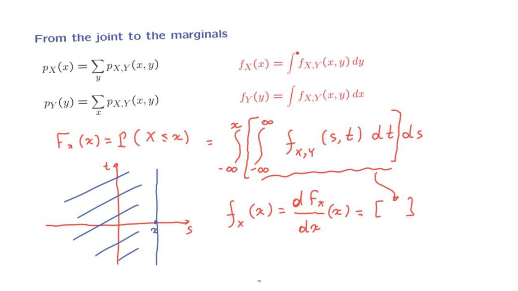
If here is the value of little x, then we’re talking about the set of all pairs x, y, for which the x component is less than or equal to a certain number.
So we need to integrate over this two-dimensional set the joint density.
So it will be a double integral of the joint density over this particular two-dimensional set.
Now, since we’ve used the symbol x here to mean something specific, let us use different symbols for the dummy variables that we will use in the integration.
And we need to integrate with respect to the two variables, let’s say with respect to t and with respect to s.
The variable t can be anything.
So it ranges from minus infinity to infinity.
But the variable s, the first argument, ranges from minus infinity up to this point, which is x.
Think of this double integral as an integral with respect to the variable s of this complicated function inside the brackets.
Now, to find the density of X, all we need to do is to differentiate the CDF of X.
And when we have an integral of this kind and we differentiate with respect to the upper limit of the integration, what we are left with is the integrand.
That is this expression here.
It is an integral with respect to the second variable.
And it’s an integral over the entire space, from minus infinity to plus infinity.
Here is an example.
The simplest kind of a joint PDF is a PDF of that is constant on a certain set, S, and is 0 outside that set.
So the overall probability, one unit of probability, is spread uniformly over that set.
Because the total volume under the joint PDF must be equal to 1, the height of the PDF must be equal to 1 over the area.
To calculate the probability of a certain set A, we want to ask how much volume is sitting on top of that set.
And because in this case, the PDF is constant, we need to take the height of the PDF times the relevant area.
What is the relevant area? Well, actually, the PDF is 0 outside the set S.
So the relevant area is only this part here, which is the intersection of the two sets, S and A.
So the total volume sitting on top of this little set is going to be the base, the area of the base, which is the area of A intersection S times the height of the PDF at those places.
Now, the height of the PDF is 1 over the area of S.
So this is the formula for calculating the probability of a certain set, A.
Let’s now look at a specific example.
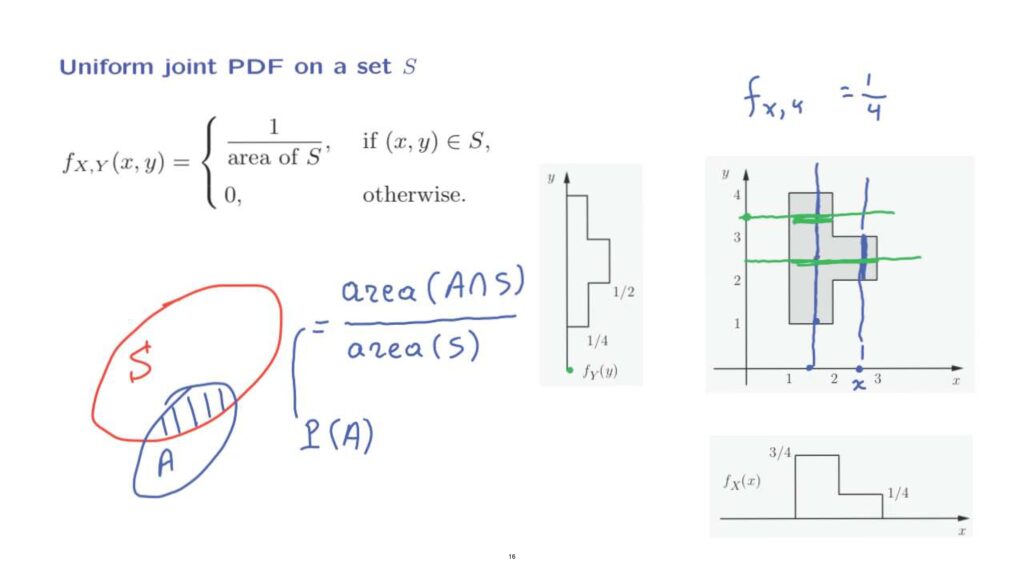
Suppose that we have a uniform PDF over this particular set, S.
This set has an area that is equal to 4.
It consists of four units rectangles arranged next to each other.
So the height of the joint PDF in this example is going to be 1/4.
It is one 1/4 on that set, but of course, it’s going to be 0 outside that set.
We can now find the marginal PDF at some particular x.
So we can fix a particular value of x, let’s say this one.
To find the value of the marginal PDF, we need to integrate over y along that particular line.
And the integral is going to have a contribution only on that segment.
On that segment, the value of the joint PDF is 1/4.
And we’re integrating over an interval that has a length of one.
So the integral is going to be equal to 1/4.
But if x is somewhere around here, as we integrate over that line, we integrate the value of 1/4, the value of the PDF, over an interval that has a length equal to 3.
And so the result turns out to be 3/4.
There’s a similar calculation for the marginal PDF of y.
For any particular value of little y, to find the marginal PDF, we integrate along this line the joint PDF.
The joint PDF is 0 out here.
It’s nonzero only on that interval.
And on that interval, it has a value of 1/4.
And the interval has a length of 1, so the integral is going to end up equal to 1/4.
But if we were to take a line somewhere here, we integrate the value of 1/4 over an interval of length 2.
And so the result would be 1/2.
So we have recovered from the joint PDF the marginal PDF of X and also the marginal PDF of Y.