In this segment, we pursue two themes.
Every concept has a conditional counterpart.
We know about PDFs, but if we live in a conditional universe, then we deal with conditional probabilities.
And we need to use conditional PDFs.
The second theme is that discrete formulas have continuous counterparts in which summations get replaced by integrals, and PMFs by PDFs.
So let us recall the definition of a conditional PMF, which is just the same as an ordinary PMF but applied to a conditional universe.
In the same spirit, we can start with a PDF, which we can interpret, for example, in terms of probabilities of small intervals.
If we move to a conditional model in which event A is known to have occurred, probabilities of small intervals will then be determined by a conditional PDF, which we denote in this manner.
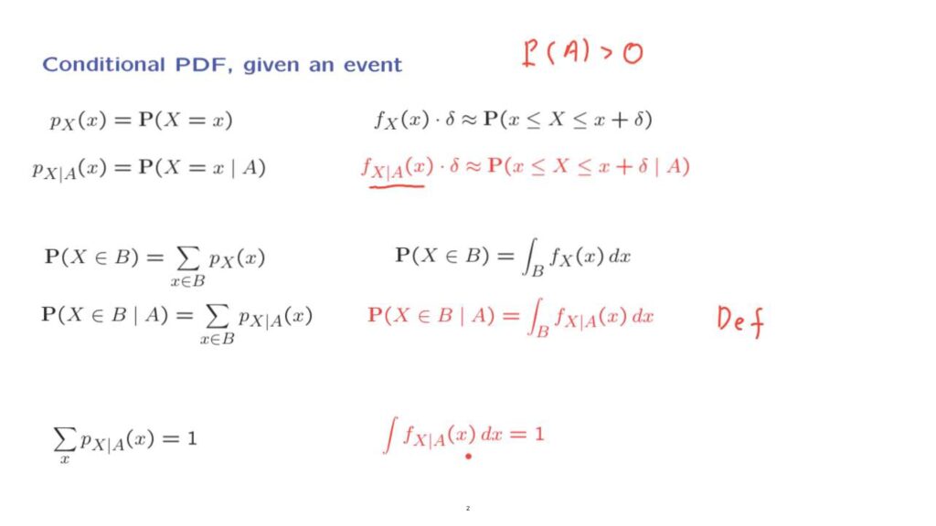
Of course, we need to assume throughout that the probability of the conditioning event is positive so that conditional probabilities are well-defined.
Let us now push the analogy further.
We can use a PMF to calculate probabilities.
The probability that X takes [a] value in a certain set is the sum of the probabilities of all the possible values in that set.
And a similar formula is true if we’re dealing with a conditional model.
Now, in the continuous case, we use a PDF to calculate the probability that X takes values in a certain set.
And by analogy, we use a conditional PDF to calculate conditional probabilities.
We can take this relation here to be the definition of a conditional PDF.
So a conditional PDF is a function that allows us to calculate probabilities by integrating this function over the event or set of interest.
Of course, probabilities need to sum to 1.
This is true in the discrete setting.
And by analogy, it should also be true in the continuous setting.
This is just an ordinary PDF, except that it applies to a model in which event A is known to have occurred.
But it still is a legitimate PDF.
It has to be non-negative, of course.
But also, it needs to integrate to 1.
When we condition on an event and without any further assumption, there’s not much we can say about the form of the conditional PDF.
However, if we condition on an event of a special kind, that X takes values in a certain set, then we can actually write down a formula.
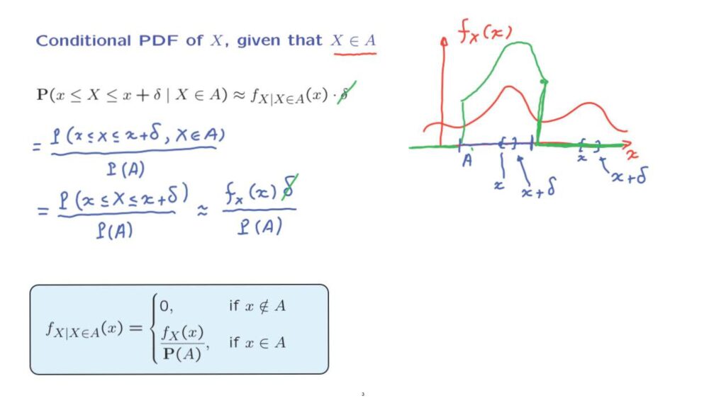
So let us start with a random variable X that has a given PDF, as in this diagram.
And suppose that A is a subset of the real line, for example, this subset here.
What is the form of the conditional PDF? We start with the interpretation of PDFs and conditional PDFs in terms of probabilities of small intervals.
The probability that X lies in a small interval is equal to the value of the PDF somewhere in that interval times the length of the interval.
And if we’re dealing with conditional probabilities, then we use the corresponding conditional PDF.
To find the form of the conditional PDF, we will work in terms of the left-hand side in this equation and try to rewrite it.
Let us distinguish two cases.
Suppose that little X lies somewhere out here, and we want to evaluate the conditional PDF at that point.
So trying to evaluate this expression, we consider a small interval from little x to little x plus delta.
And now, let us write the definition of a conditional probability.
A conditional probability, by definition, is equal to the probability that both events occur divided by the probability of the conditioning event.
Now, because the set A and this little interval are disjoint, these two events cannot occur simultaneously.
So the numerator here is going to be 0.
And this will imply that the conditional PDF is also going to be 0.
This, of course, makes sense.
Conditioned on the event that X took values in this set, values of X out here cannot occur.
And therefore, the conditional density out here should also be 0.
So the conditional PDF is 0 outside the set A.
And this takes care of one case.
Now, the second case to consider is when little x lies somewhere inside here inside the set A.
And in that case, our little interval from little x to little x plus delta might have this form.
In this case, the intersection of these two events, that X lies in the big set and X lies in the small set, the intersection of these two events is the event that X lies in the small set.
So the numerator simplifies just to the probability that the random variable X takes values in the interval from little x to little x plus delta.
And then we rewrite the denominator.
Now, the numerator is just an ordinary probability that the random variable takes values inside a small interval.
And by our interpretation of PDFs, this is approximately equal to the PDF evaluated somewhere in that small interval times delta.
At this point, we notice that we have deltas on both sides of this equation.
By cancelling this delta with that delta, we finally end up with a relation that the conditional PDF should be equal to this expression that we have here.
So to summarize, we have shown a formula for the conditional PDF.
The conditional PDF is 0 for those values of X that cannot occur given the information that we are given, namely that X takes values at that interval.
But inside this interval, the conditional PDF has a form which is proportional to the unconditional PDF.
But it is scaled by a certain constant.
So in terms of a picture, we might have something like this.
And so this green diagram is the form of the conditional PDF.
The particular factor that we have here in the denominator is exactly that factor that is required, the scaling factor that is required so that the total area under the green curve, under the conditional PDF is equal to 1.
So we see once more the familiar theme, that conditional probabilities maintain the same relative sizes as the unconditional probabilities.
And the same is true for conditional PMFs or PDFs, keeping the same shape as the unconditional ones, except that they are re-scaled so that the total probability under a conditional PDF is equal to 1.
We can now continue the same story and revisit everything else that we had done for discrete random variables.
For example, we have the expectation of a discrete random variable and the corresponding conditional expectation, which is just the same kind of object, except that we now rely on conditional probabilities.
Similarly, we can take the definition of the expectation for the continuous case and define a conditional expectation in the same manner, except that we now rely on the conditional PDF.
So this formula here is the definition of the conditional expectation of a continuous random variable given a particular event.
We have a similar situation with the expected value rule, which we have already seen for discrete random variables in both of the unconditional and in the conditional setting.
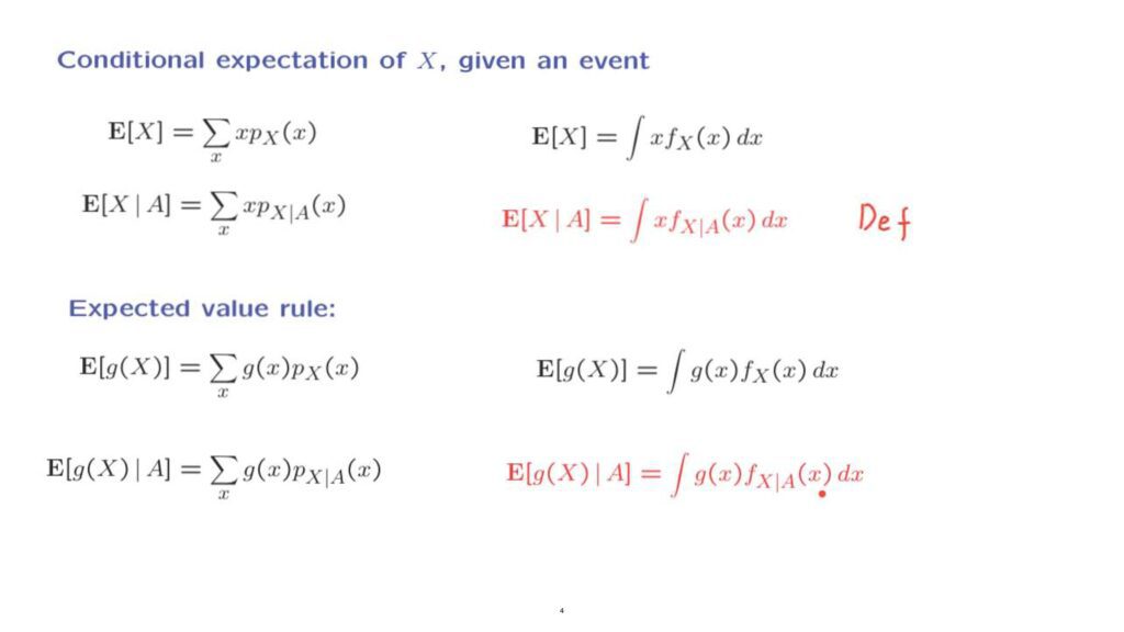
We have a similar formula for the continuous case.
And at this point, you can guess the form that the formula will take in the continuous conditional setting.
This is the expected value rule in the conditional setting, and it is proved exactly the same way as for the unconditional continuous setting, except that here in the proof, we need to work with conditional probabilities and conditional PDFs, instead of the unconditional ones.
So to summarize, there is nothing really different when we condition on an event in the continuous case compared to the discrete case.
We just replace summations with integrations.
And we replace PMFs by PDFs.