We will now study a problem which is quite difficult to approach in a direct brute force manner but becomes tractable once we break it down into simpler pieces using several of the tricks that we have learned so far.
And this problem will also be a good opportunity for reviewing some of the tricks and techniques that we have developed.
The problem is the following.
There are n people.
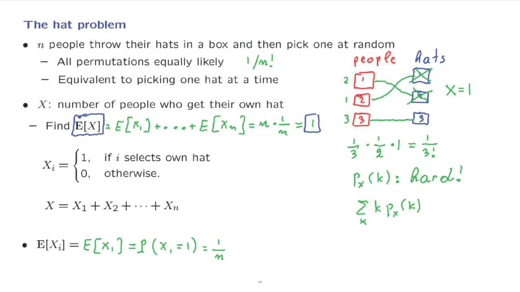
And let’s say for the purpose of illustration that we have 3 people, persons 1, 2, and 3.
And each person has a hat.
They throw their hats inside a box.
And then each person picks a hat at random out of that box.
So here are the three parts.
And one possible outcome of this experiment is that person 1 ends up with hat number 2, person 2 ends up with hat number 1, person 3 ends up with hat number 3.
We could indicate the hats that each person got by noting here the numbers associated with each person, the hat numbers.
And notice that this sequence of numbers, which is a description of the outcome of the experiment, is just a permutation of the numbers 1, 2, 3 of the hats.
So we permute the hat numbers so that we can place them next to the person that got each one of the hats.
In particular, we have n factorial possible outcomes.
This is the number of possible permutations.
What does it mean to pick hats at random? One interpretation is that every permutation is equally likely.
And since we have n factorial permutations, each permutation would have a probability of 1 over n factorial.
But there’s another way of describing our model, which is the following.
Person 1 gets a hat at random out of the three available.
Then person 2 gets a hat at random out of the remaining hats.
Then person 3 gets the remaining hat.
Each time that there is a choice, each one of the available hats is equally likely to be picked as any other hat.
Let us calculate the probability, let’s say, that this particular permutation gets materialized.
The probability that person 1 gets hat number 2 is 1/3.
Then we’re left with two hats.
Person 2 has 2 hats to choose from.
The probability that it picks this particular hat is going to be 1/2.
And finally, person 3 has only 1 hat available, so it will be picked with probability 1.
So the probability of this particular permutation is one over 3 factorial.
But you can repeat this argument and consider any other permutation, and you will always be getting the same answer.
Any particular permutation has the same probability, one over 3 factorial.
The same argument goes through for the case of general n, n people and n hats.
And we will find that any permutation will have the same probability, 1/n factorial.
Therefore, the process of picking one hat at a time is probabilistically identical to a model in which we simply state that all permutations are equally likely.
Now that we have described our model and our process and the associated probabilities, let us consider the question we want to answer.
Let X be the number of people who get their own hat back.
For example, for the outcome that we have drawn here, the only person who gets their own hat back is person 3.
And so in this case X happens to take the value of 1.
What we want to do is to calculate the expected value of the random variable X.
The problem is difficult because if you try to calculate the PMF of the random variable X and then use the definition of the expectation to calculate this sum, you will run into big difficulties.
Calculating this quantity, the PMF of X, is difficult.
And it is difficult because there is no simple expression that describes it.
So we need to do something more intelligent, find some other way of approaching the problem.
The trick that we will use is to employ indicator variables.
Let Xi be equal to one 1 if person i selects their own hat and 0 otherwise.
So then, each one of the Xi’s is 1 whenever a person has selected their own hat.
And by adding all the 1’s that we may get, we obtain the total number of people who have selected their own hats.
This makes things easier, because now to calculate the expected value of X it’s sufficient to calculate the expected value of each one of those terms and add the expected values, which we’re allowed to do because of linearity.
So let’s look at the typical term here.
What is the expected value of Xi? If you consider the first description or our model, all permutations are equally likely, this description is symmetric with respect to all of the persons.
So the expected value of Xi should be the same as the expected value of X1.
Now, to calculate the expected value of X1, we will consider the sequential description of the process in which 1 is the first person to pick a hat.
Now, since X1 is a Bernoulli random variable that takes values 0 or 1, the expected value of X1 is just the probability that X1 is equal to 1.
And if person 1 is the first one to choose a hat, that person has probability 1/n of obtaining the correct hat.
So each one of these random variables has an expected value of 1/n.
The expected value of X by linearity is going to be the sum of the expected values.
There is n of them.
Each expected value is 1/n.
And so the final answer is 1.
This is the expected value of the random variable X.
Let us now move and try to calculate a more difficult quantity, namely, the variance of X.
How shall we proceed? Things would be easiest if the random variables Xi were independent.
Because in that case, the variance of X would be the sum of the variances of the Xi’s.
But are the Xi’s independent? Let us consider a special case.
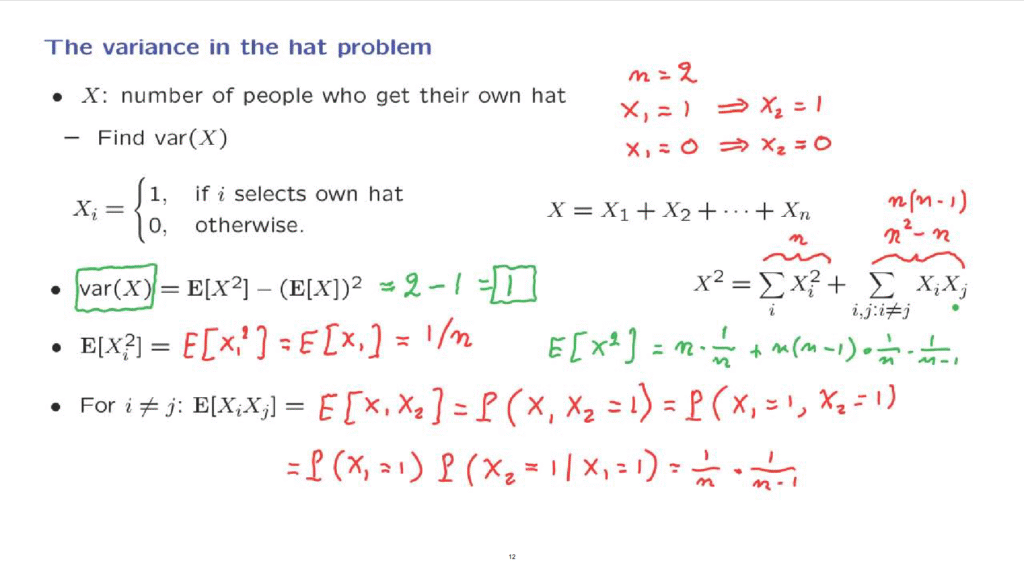
Suppose that we only have two persons and that I tell you that the first person got their own hat back.
In that case, the second person must have also gotten their own hat back.
If, on the other hand, person 1 did not to get their own hat back, then person 2 will not get their own hat back either.
Because in this scenario, person 1 gets hat 2, and that means that person 2 gets hat 1.
So we see that knowing the value of the random variable X1 tells us a lot about the value of the random variable X2.
And that means that the random variables X1 and X2 are dependent.
More generally, if I were to tell you that the first n minus 1 people got their own hats back, then the last remaining person will have his or her own hat available to be picked.
That’s going to be the only available hat.
And then person n we also get their hat back.
So we see that the information about some of the Xi’s gives us information about the remaining Xn.
And again, this means that the random variables are dependent.
Since we do not have independence, we cannot find the variance by just adding the variances of the different random variables.
But we need to do a lot more work in that direction.
In general, whenever we need to calculate variances, it is usually simpler to carry out the calculation using this alternative form for the variance.
So let us start towards a calculation of the expected value of X squared.
Now the random variable X squared, by simple algebra, is this expression times itself.
And by expanding the product we get all sorts of cross terms.
Some of these cross terms will be of the type X1 times Xi or X2 times X2.
These will be terms of this form, and there is n of them.
And then we get cross terms, such as X1 times X2, X1 times X3, X2 times X1, and so on.
How many terms do we have here? Well, if we have n terms multiplying n other terms we have a total of n squared terms.
n are already here, so the remaining terms, which are the cross terms, will be n squared minus n.
Or, in a simpler form, it’s n times n minus 1.
So now how are we going to calculate the expected value of X squared? Well, we will use linearity of expectations.
So we need to calculate the expected value of Xi squared, and we also need to calculate the expected value of Xi Xj when i is different from j.
Let us start with Xi squared.
First, if we use the symmetric description of our model, all permutations are equally likely, then all persons play the same role.
There’s symmetry in the problem.
So Xi squared has the same distribution as X1 squared.
Then, X1 is a 0-1 random variable, a Bernoulli random variable.
So X1 squared will always take the same numerical value as the random variable X1.
This is a very special case which happens only because a random variable takes values in {0, 1}.
And 0 squared is the same as 0.
1 squared is the same as 1.
This expected value is something that we have already calculated, and it is 1/n.
Let us now move to the calculation of the expectation of a typical term inside the sum.
So let i be different than j, and look at the expected value of Xi Xj.
Once more, because of the symmetry of the probabilistic model, it doesn’t matter which i and j we are considering.
So we might as well consider the product of X1 with X2.
Now, X1 and X2 take values 0 and 1.
And the product of the two also takes values 0 and 1.
So this is a Bernoulli random variable, and so the expectation of that random variable is just the probability that this random variable is equal to 1.
But for the product to be equal to 1, the only way that this can happen is if both of these random variables happen to be equal to 1.
Let us now turn to the sequential description of the model.
The probability that the first person gets their own hat back and the second person gets their own hat back is the probability that the first one gets their own hat back, and then multiplied by the conditional probability that the second person gets their own hat back, given that the first person got their own hat back.
What are these probabilities? The probability that a person gets their own hat back is 1/n.
Given that person 1 got their own hat back, person 2 is faced with a situation where there are n minus 1 available hats.
And one of those is that person’s hat.
So the probability that person 2 will also pick his or her own hat is 1 over n minus 1.
Now we are in a position to calculate the expected value of X squared.
The expected value of X squared consists of the sum of n expected values, each one of which is equal to 1/n plus so many expected values, because we have so many terms, each one of which, by this calculation, is 1/n times 1 over n minus 1.
And we see that we get cancellations here.
And we obtain 1 plus 1, which is equal to 2.
On the other hand we have this term that we need to subtract.
We found previously that the expected value of X is equal to 1.
So we need to subtract 1.
And the final answer to our problem is that the variance of X is also equal to 1.
So what we saw in this problem is that we can deal with quite complicated models, but by breaking them down into more manageable pieces, first break down the random variable X as a sum of different random variables, then taking the square of this and break it down into a number of different terms, and then by considering one term at a time, we can often end up with the solutions or the answers to problems that would have been otherwise quite difficult.