We have already introduced the concept of the conditional PMF of a random variable, X, given an event A.
We will now consider the case where we condition on the value of another random variable Y.
That is, we let A be the event that some other random variable, Y, takes on a specific value, little y.
In this case, we’re talking about a conditional probability of the form shown here.
The conditional probability– that X takes on a specific value, given that the random variable Y takes on another specific value.
And we use this notation to indicate those conditional probabilities.
As usual, the subscripts indicate the situation that we’re dealing with.
That is, we’re dealing with the distribution of the random variable X and we’re conditioning on values of the other random variable, Y.
Using the definition now of conditional probabilities this can be written as the probability that both events happen divided by the probability of the conditioning event.
We can turn this expression into PMF notation.
And this leads us to this definition of conditional PMFs.
The conditional PMF is defined to be the ratio of the joint PMF– this is the probability that we have here– by the corresponding marginal PMF.
And this is the probability that we have here.
Now, remember that conditional probabilities are only defined when the conditioning event has a positive probability, when this denominator is positive.
Similarly, the conditional PMF will only be defined for those little y that have positive probability of occurring.
Now, the conditional PMF is a function of two arguments, little x and little y.
But the best way of thinking about the conditional PMF is that we fix the value, little y, and then view this expression here as a function of x.
As a function of x, it gives us the probabilities of the different x’s that may occur in the conditional universe.
And these probabilities must, of course, sum to 1.
Again, we’re keeping y fixed.
We live in a conditional universe where y takes on a specific value.
And here we have the probabilities of the different x’s in that universe.
And these sum to 1.
Note that if we change the value of little y, we will, of course, get a different conditional PMF for the random variable X.
So what we’re really dealing with in this instance is that we have a family of conditional PMFs, one conditional PMF for every possible value of little y.
And for every possible value of little y, we have a legitimate PMF who’s values add to 1.
Let’s look at an example.
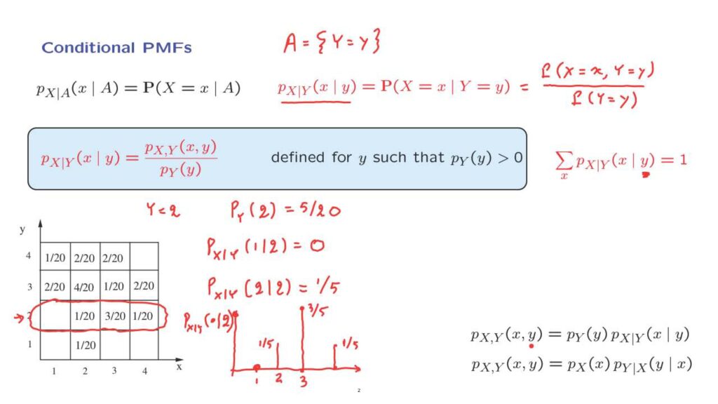
Consider the joint PMF given in this table.
Let us condition on the event that Y is equal to 2, which corresponds to this row in the diagram.
We need to know the value of the marginal at this point, so we start by calculating the probability of Y at value 2.
And this is found by adding the entries in this row of the table.
And we find that this is 5 over 20.
Then we can start calculating entries of the conditional PMF.
So for example, the probability that X takes on the value of 1 given that Y takes the value of 2, it is going to be this entry, which is 0, divided by 5/20, which gives us 0.
We can find the next entry, the probability of X taking the value of 2, given that Y takes the value of 2 will be this entry, 1/20 divided by 5/20.
So it’s going to be 1/5.
And we can continue with the other two entries.
And we can actually even plot the result once we’re done.
And what we have is that at 1, we have a probability of 0.
At 2, we have a probability of 1/5.
At 3, we have a probability of 3/20 divided 5/20, which is 3/5.
And at 4, we have, again, a probability of 1/5.
So what we have plotted here is the conditional PMF.
It’s a PMF in the variable x, where x ranges over the possible values, but where we have fixed the value of y to be equal to 2.
Now, we could have found this conditional PMF even faster without doing any divisions by following the intuitive argument that we have used before.
We live in this conditional universe.
We have conditioned on Y being equal to 2.
The conditional probabilities will have the same proportions as the original probabilities, except that they needed to be scaled so that they add to 1.
So they should be in the proportions of 0, 1, 3, 1.
And for these to add to 1, we need to put everywhere a denominator of 5.
So the proportions are indeed 0, 1, 3, and 1.
Pictorially, the conditional PMF has the same form as the corresponding slice of the joint PMF, except, again, that the entries of that slice are renormalized so that the entries add to 1.
And finally, an observation– we can take the definition of the conditional PMF and turn it around by moving the denominator to the other side and obtain a formula, which is a version of the multiplication rule.
The probability that X takes a value little x and Y takes a value little y is the product or the probability that Y takes this particular value times the conditional probability that X takes on the particular value little x, given that Y takes on the particular value little y.
We also have a symmetrical relationship if we interchange the roles of X and Y.
As we discussed earlier in this course, the multiplication rule can be used to specify probability models.
One way of modeling two random variables is by specifying the joint PMF.
But we now have an alternative, indirect, way using the multiplication rule.
We can first specify the distribution of Y and then specify the conditional PMF of X for any given value of little y.
And this completely determines the joint PMF, and so we have a full probability model.
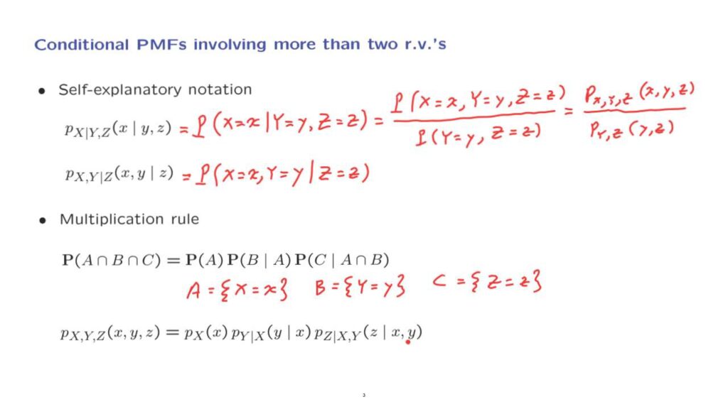
We can also provide similar definitions of conditional PMFs for the case where we’re dealing with more than two random variables.
In this case, notation is pretty self-explanatory.
By looking at this expression here, you can probably guess that this stands for the probability that random variable X takes on a specific value, conditional on the random variables Y and Z taking on some other specific values.
Using the definition of conditional probabilities, this is the probability that all events happen divided by the probability of the conditioning event, which, in our case, is the event that Y takes on a specific value and simultaneously, Z takes another specific value.
In PMF notation, this is the ratio of the joint PMF of the three random variables together, divided by the joint PMF of the two random variables Y and Z.
As another example, we could have an expression like this, which, again, stands for the probability that these two random variables take on specific values, conditional on this random variable taking on another value.
Finally, we can have versions of the multiplication rule for the case where we’re dealing with more than two random variables.
Recall the usual multiplication rule.
For three events happening simultaneously, let’s apply this multiplication rule for the case where the event, A, stands for the event that the random variable X takes on a specific value.
Let B be the event that Y takes on a specific value, and C be the event that the random variable Z takes on a specific value.
Then we can take this relation, the multiplication rule, and translate it into PMF notation.
The probability that all three events happen is equal to the product of the probability that the first event happens.
Then we have the conditional probability that the second event happens given that the first happened, times the conditional probability that the third event happens– this one– given that the first two events have happened.