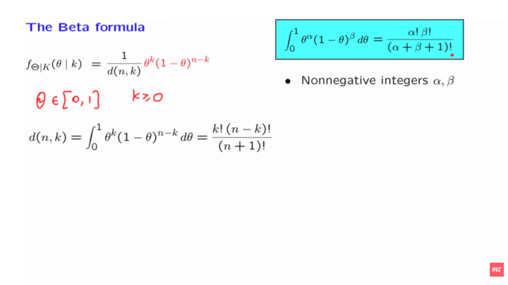
In the context of the problem of estimating the unknown bias of a coin, we encountered this distribution, which is known as a Beta distribution.
It’s a probability density for a random variable, Theta, that takes values in the interval from 0 to 1.
So this formula is valid for thetas in this range.
And k here is a non-negative integer.
Now, this coefficient here, d(n,k), is a normalizing constant, which is needed so that this is a legitimate PDF, that it integrates to 1.
And so in particular, d needs to be equal to the integral of what we have in the numerator.
This is the choice that makes this whole expression integrate to 1.
And this integral is calculated and can be found to be equal to this particular expression.
How do we derive this expression?
One way is to carry out a long exercise in calculus.
We have this integral here.
You might either expand it and then integrate and collect terms, or you could try to demonstrate this equality by applying integration by parts.
But this is complicated.
Is there some simple way of arguing and deriving this expression?
We will see that there is a very simple probabilistic argument for deriving this equality.
What we will actually derive is this same equality, but in slightly different notation.
Instead of k, we will use alpha.
Instead of n minus k, we will use beta.
So here we have alpha factorial times beta factorial.
In the denominator, we have the sum of these two coefficients plus 1, so this corresponds to alpha plus beta plus 1 factorial.
This is what we want to demonstrate.
What we will do will be to consider the following setting.
We start with alpha plus beta plus 1, that many independent random variables that are uniform on the unit interval, and we will consider the following event and its probability.
This is the probability that these random variables happen to be ordered in some particular order.
Let us call this event A, so this is the probability of A.
Now, this probability is not hard to calculate.
We have alpha plus beta plus 1 random variables– independent, identically distributed.
By symmetry, any particular way of ordering these random variables is equally likely.
How many ways are there to order alpha plus beta plus 1 random variables?
It’s the factorial of the number of items that we’re trying to order.
We’re talking about the probability of a particular permutation, so this probability is equal to 1 over the number of permutations of alpha plus beta plus 1 objects.
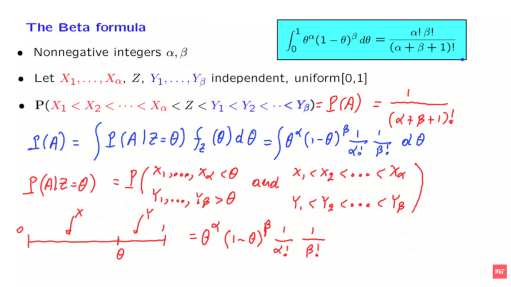
So this is one expression for the probability of this event A.
Now, we’re going to calculate this probability in a different way.
What we will do is we’re going to apply the total probability theorem.
We’re going to condition on Z.
We’re going to calculate the conditional probability of A given that Z takes a specific value, and then weigh those probabilities according to the probability density of the random variable Z.
So this is just the total probability theorem applied to this particular context.
And now to make progress, what we will need to do is to find this conditional probability.
We fix a constant little theta, and we want the probability that this event happens.
What is this event?
It is the event that all of the X’s fall inside this interval, all the Y’s fall inside this interval, and furthermore, the X’s are sorted and the Y’s are sorted.
So let us write this out.
It’s the probability that all of the X’s happen to be less than theta, all the Y’s happen to be bigger than theta, and also, not just that, but the X’s are sorted, and furthermore, the Y’s are sorted as well.
Clearly, if I give you the value of theta so that Z is equal to theta, for this event to happen, we must have all these events here happen as well.
So now, let us try to calculate the probability of this event.
We’re going to use the multiplication rule.
First, take the probability of this event and then the conditional probability of that event.
The X’s and the Y’s are independent, so we can take the probability of this event and then multiply with the probability of this event involving the Y’s.
How about the probability of this event, that all of the X’s are less than theta?
Since the X’s are independent, this is going to be equal to the probability that X1 is less than theta.
What is this probability?
Since X1 is uniform on the unit interval and this is theta, the probability of falling in this interval is equal to theta.
Times the probability that X2 is less than theta.
This probability is, again, theta and so on.
We have alpha many terms of that kind, so this probability that all of these random variables are less theta is equal to theta to the power of alpha.
Similarly, about the Y’s.
For any particular Y, the probability that it falls in this interval is equal to the length of this interval, which is 1 minus theta.
This is the probability for each one of the Y’s.
There’s beta many Y’s.
The Y’s are independent.
So the probability that all of them fall in this interval is going to be this number to the power of beta.
So suppose that I told you that all the X’s are less than theta, and then I ask you, given this information, what is the probability that the X’s that you got are arranged in this particular order?
Now, because of the complete symmetry of the problem, even if I told you that all the X’s fall inside this interval, any order of the X’s is equally likely.
So the probability of this particular order is going to be 1 over the number of possible orderings.
How many ways are there that alpha items can be ordered?
There are alpha factorial possible orderings, so the probability that I obtain one particular ordering is 1 over alpha factorial.
And similarly, if I tell you that the Y’s all fell in this interval by symmetry, the probability of a particular order is going to be 1 over the [number of possible] orders, which is beta factorial.
All right.
So we have this conditional probability, and now we can go back to this formula and substitute, and what we obtain is the integral of this expression, theta to the alpha, 1 minus theta [to the] beta, 1 over alpha factorial times 1 over beta factorial.
Then we have the density of Z, but since Z is uniform, the density is equal to 1.
And then we have a factor of d theta.
So what have we achieved?
We calculated the probability of the event A in two different ways, and we got two seemingly different answers.
But these two answers have to agree.
Therefore, this expression is equal to that expression.
And now if you take this factor, 1 over alpha factorial times 1 over beta factorial, and send it to the other side of the equation, what we obtain is exactly the formula that we wished to derive.
This example is an instance of the following.
There are certain formulas in mathematics that are somewhat complicated to derive, and their derivations using, for example, calculus are quite unintuitive.
But once you interpret the various terms that appear in such a relation in a probabilistic way, you can sometimes find very easy derivations and explanations why such a formula has to be true.