In this segment, we will look at the famous example, which was posed by Comte de Buffon– a French naturalist– back in the 18th century.
And it marks the beginning of a subject that is known as the subject of geometric probability.
The problem is pretty simple.
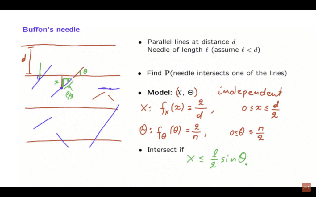
We have the infinite plane, and we draw lines that are parallel to each other.
And they’re spaced apart d units.
So this distance here is d.
And the same for all the other lines.
We take a needle that has a certain length– l– and we throw it at random on the plane.
So the needle might fall this way, so that it doesn’t cross any line, or it might fall this way, so that it ends up crossing one of the lines.
If the needle is long enough, it might actually even end up crossing two of the lines.
But we will make the assumption that the length of the needle is less than the distance between the two– between two adjacent lines, so that we’re going to have either this configuration, or that configuration.
So in this setting, we’re interested in the question of how likely is it that the needle is going to intersect one of the lines if the needle is thrown completely at random? We will answer this question, and we will proceed as follows.
First, we need to model the experiment– the probabilistic experiment– mathematically.
That is, we need to define an appropriate sample space, define some relevant random variables, choose an appropriate probability law, identify the event of interest, and then calculate.
Let us see what it takes to describe a typical outcome of the experiment.
Suppose that the needle fell this way, so that the nearest line is the one above.
And let us mark here the center of the needle.
One quantity of interest is this vertical distance between the needle and the nearest line.
Let us call this quantity x.
We’re using here a lowercase x, because we’re dealing with a numerical value in one particular outcome of the experiment.
But we think of this x as being the realization of a certain random variable that we will denote by capital X.
What else does it take to describe the needle? Suppose that the needle had fallen somewhere so that it is at the same vertical distance from the nearest line, but it has an orientation of this kind.
This orientation compared to that one should make a difference.
Because when it falls that way, it’s more likely that it’s going to cut the next line as opposed to this case.
So the angle that the needle is making with the parallel lines should also be relevant.
So let us give a name to that particular angle.
So let’s extend that line until it crosses one of the lines.
And let us give a name to this angle, and call it theta.
So if I tell you x and theta, you know how far away the needle is from the nearest line, and at what angle it is.
It looks like these are two useful variables to describe the outcome of the experiment, so let us try working with these.
So our model is going to involve two random variables defined the way we discussed it just now.
What is the range of these random variables? Since we took x to be the distance from the nearest line, and the lines are d units apart, this means that x is going to be somewhere between 0 and d over 2.
How about theta? So the needle makes two angles with the part of the line.
It’s this angle, and the complimentary one.
Which one do we take? Well, we use a convention that theta is defined as the acute angle that the direction of the needle is making with the lines, so that theta will vary over a range from 0 to pi over 2.
And our sample space for the experiments who will be the set of all pairs of x and theta, that satisfy these two conditions.
These will be the possible x’s and thetas.
Having defined the sample space, next we need to define a probability law.
At this point, we do not want to make any arbitrary assumptions.
We only have the words completely at random to go by.
But what do these words mean? We will interpret them to mean that there are no preferred x values, so that all x values are- in some sense– equally likely.
So we’re going to assume that x is a uniform random variable.
Since it is uniform, it’s going to be a constant over this range.
And in order to integrate to 1, that constant will have to be 2 over d.
And we understand that the PDF of x is 0 outside that range.
Similarly for theta, we do not want to assume that some orientations are more likely than other orientations.
So we will again assume a uniform probability distribution.
And therefore, that PDF must be equal to 2 over pi for theta’s over this particular range.
So far, we have specified the marginal PDFs of each one of the two random variables.
How about the adjoined PDF? In order to have a complete model, we need to have a joint PDF in our hands.
Here, we’re going to make the assumption that x and theta are independent of each other.
And in that case, the joint PDF is determined by just taking the product of the marginal PDFs.
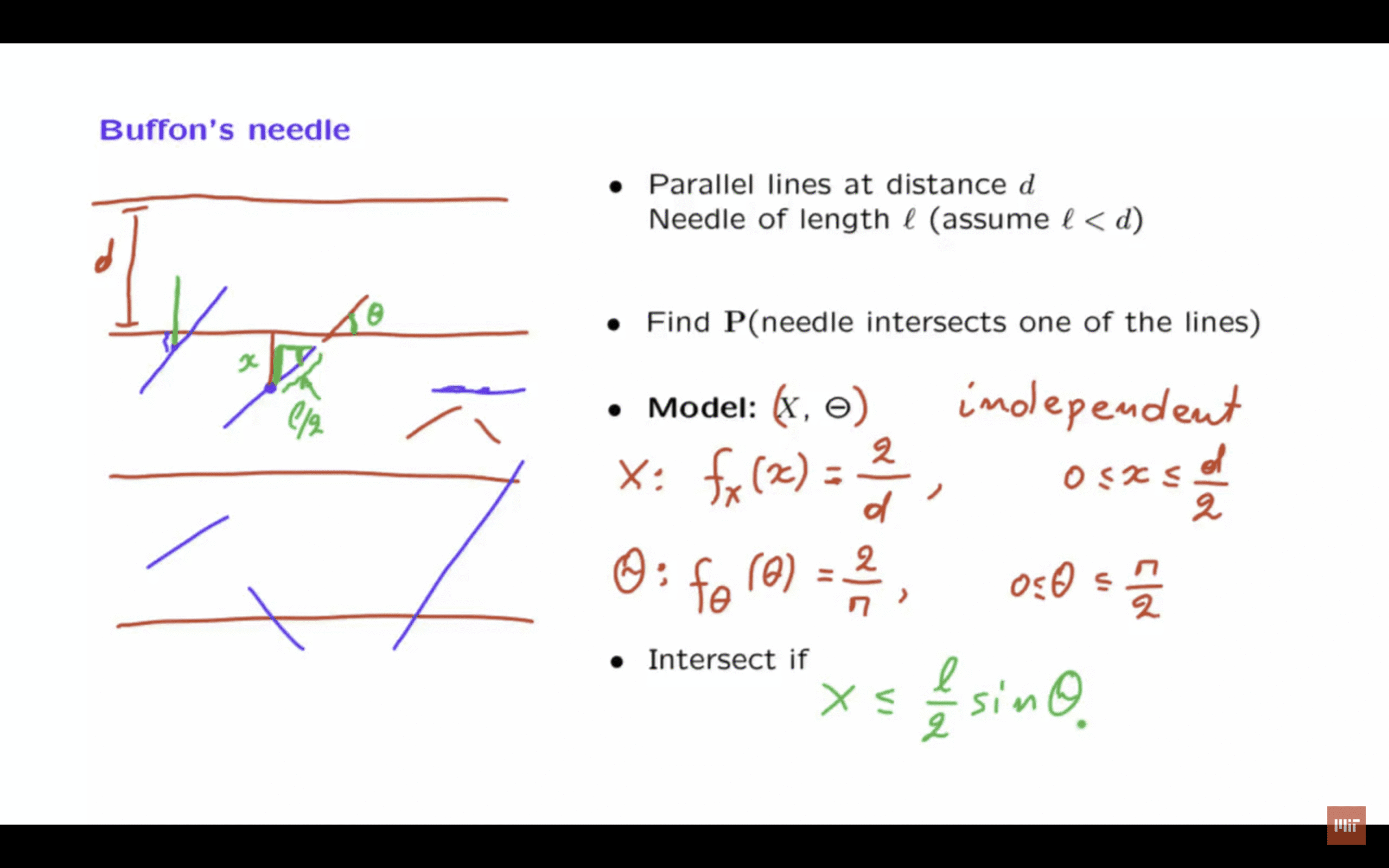
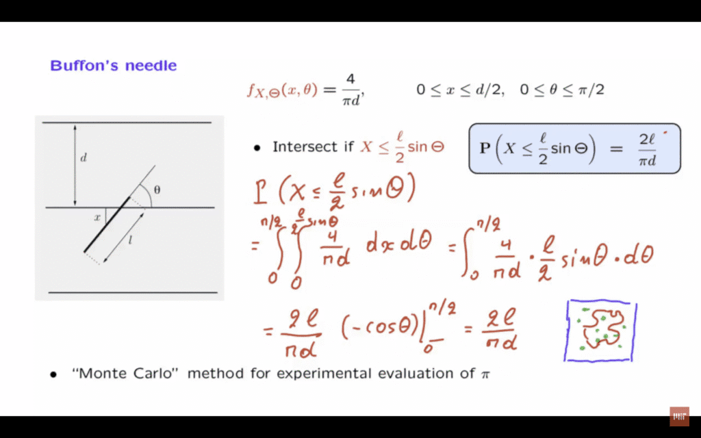
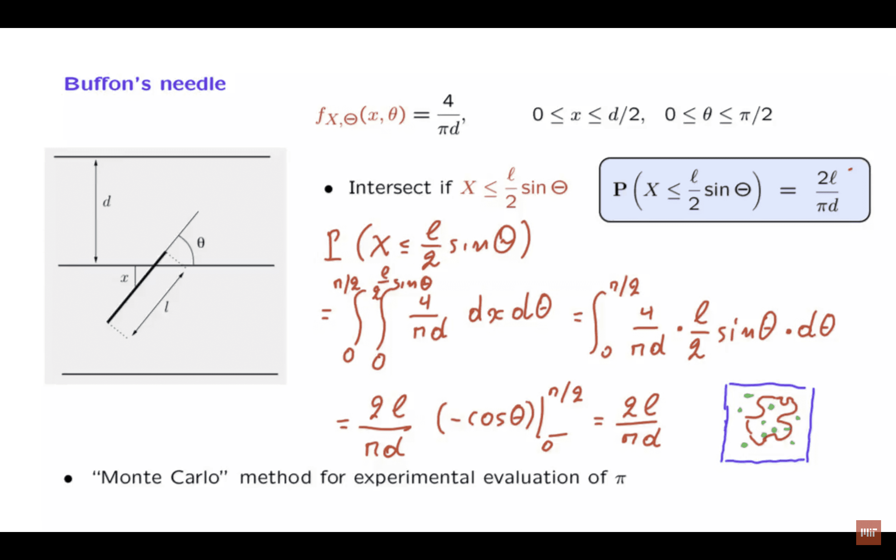
So the joint PDF is going to be equal to 4 divided by pi times d.
By this point, we have completely specified a probabilistic model.
We have made some assumptions, which you might even consider arbitrary.
But these assumptions are a reasonable attempt at capturing the idea that the needle is thrown completely at random.
This completes the subjective part– the modeling part.
The next step is much more streamlined.
There’s not going to be any choices.
We just need to consider the event of interest, express it in terms of the random variables that we have in our hands, and then use the probability model that we have to calculate the probability of this particular event.
So let us identify the event of interest.
When will the needle intersect the nearest line? This will depend on the following.
We can look at the vertical extent of the needle.
By vertical extent, I mean the following.
Let’s see how far the needle goes in the vertical direction, which is the length of this green segment here.
In this example, the vertical extent of the needle is less than the distance from the next line.
And we do not have an intersection.
If the figure was something like this, the vertical extent of the needle would have been that, but x would have been just this little segment.
The vertical extent is bigger than x and the needle intersects the line.
So we have an intersection if and only if the vertical extent– which is this vertical green segment– is larger than the distance x.
Or equivalently, if x is less than the vertical extent.
So we will have an intersection if x is less than or equal to the vertical extent of the needle.
Now, how big is this vertical extent? Let’s use some trigonometry here.
This angle here is theta, so this angle here is also theta.
Here, we have a right triangle and the hypotenuse of this triangle is l over 2.
This angle is theta, therefore this vertical segment is equal to l over 2 times sine theta.
So this is the geometrical condition that describes the event that the needle intersects the nearest line.
And all we need to do now is to calculate the probability of this event.
So here is what we have so far.
This is the picture that we had before, but drawn in a somewhat nicer way.
This is the joint PDF that we decided upon.
And we wish to calculate the probability of this particular event– that x is less than or equal to l over 2 sine theta.
How do we calculate the probability of an event that has to do with two random variables? What we do is we take the joint PDF– which in our case is four over pi d– and integrate it over the set of x’s and theta’s for which the PDF is non-zero.
So it’s only going to be over x’s and theta’s in those ranges and also, only for those x theta pairs for which the event occurs.
So what are these pairs? This event can occur with any choice of theta.
So theta is free to vary from 0 up to pi over 2.
How about x? For this event to occur, x can be anything that is non-negative as long as it is less than or equal to this number.
So the upper limit of this integration is going to be l over 2 times sine theta.
And all we need to do now is to evaluate this double integral.
Let’s start with the inner integral.
Because we’re just integrating a constant, the inner integral evaluates to the quantity that we’re integrating– the constant that we’re integrating– which is 4 times pi d times the length of the interval over which we’re integrating, which is l over 2 sine theta.
And now we need to carry out the outer integral.
Let us pull out the constants, which is this 4 with this 2 give us a 2.
We have 2l over pi d.
And then the integral from 0 to pi over 2 of sine theta.
Now the integral of sine theta is minus cosine theta.
And we need to evaluate this at 0 and pi over 2.
This turns out to be equal to 1.
So the final result is 2 l over pi d.
And this is the final answer to the problem that we have been considering.
And now, a curious thought.
Suppose that you do not know what the number pi is and all you have in your hands is your floor, lines drawn on your floor, and the needle.
And you do know the length between adjacent lines on your floor.
And you do know your length of your needle.
How can you figure out the number pi? Take your needle, throw it at random a million times, and count the frequency with which the needle ends up crossing the line.
If you believe that probabilities can be interpreted as frequencies, the frequency that you observe gives you a good estimate of this probability.
So it gives you a good estimate of this particular number.
And if you know the length of your needle and of the distance between the different lines, you can use the estimate of that number to determine the value of pi.
This is a so-called Monte Carlo method, which uses simulation to evaluate experimentally the value, in this case, of the constant pi.
Of course, for pi, we have much better ways of calculating it.
But there are many applications in engineering and in physics where certain quantities are hard to calculate, but they can be calculated using a trick of this kind by simulation.
Here’s a typical situation.
Consider the unit cube.
And for simplicity, I’m only taking a cube in two dimensions.
But in general, think of the unit cube in n dimensions, which is an object that has unit volume.
Inside that unit cube, there is a complicated subset which is described maybe by some very complicated formulas.
And you want to calculate the volume of this complicated subset.
The description of the subset is so complicated that using integration, multiple integrals, and calculus is practically impossible.
What can you do? What you can do is to start throwing at random points inside that unit cube.
So you throw points.
Some fault inside.
Some fall outside.
You count the frequency with which the points happen to be inside your set.
And as long as you’re throwing the points uniformly over the cube, then the probability of your complicated set is going to be the volume of that set.
You estimate the probability by counting the frequency with which you get points in that set.
And so, by using these observed frequencies, you can estimate the volume of a set– something that might be very difficult to do through other numerical methods.
It turns out that these days, physicists and many engineers use methods of this kind quite often and in many important applications.