We now continue our discussion of the model in which we obtain several measurements of an unknown random variable Theta in the presence of additive noise, under the same assumptions as before.
Theta and Wi are all independent random variables.
And they’re also normal.
We have seen that in this case, the posterior distribution of Theta is a normal distribution, and it takes this particular form.
We found the mean of the posterior distribution, which is also the maximum posterior probability estimate.
And it is given by this expression.
Now that we have an estimate in our hands, we can ask, how good is this estimate?
And for this, we need an appropriate performance measure.
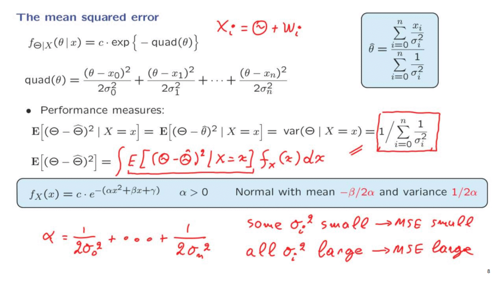
For estimation problems, a reasonable performance measure is to look at the mean value of the squared error.
But given that we have already obtained observations, what we’re interested in is the conditional mean squared error.
This is the error that’s remaining after we have seen the observations.
Now, let us notice something here.
If I tell you the value of the observations, then my estimator is completely determined.
The estimator is a random variable that processes the data and comes up with an estimate.
So although it is a random variable, once I tell you the value of the observations, the value of this random variable has been completely determined.
And so we can replace it with its actual numerical value, which is theta hat.
And it is given by this expression.
Now remember also that theta hat, the estimate that we’re using, is the mean of the posterior distribution.
In this conditional universe where we have conditioned on this information, theta hat is the mean of this random variable.
So we’re dealing with the square distance from the mean.
And then we take the expected value.
But that’s nothing but the variance of Theta in this conditional universe.
So what we’re looking for is the variance of the posterior distribution of Theta, given the observations that we have obtained.
Can we eyeball the variance by just looking at this formula for the posterior distribution?
More or less, we can.
Recall this earlier fact that if I give you a density of this form, you recognize that it is normal.
And you also recognize that the variance is determined by the coefficient that comes next to a term of the form x squared.
Now, this is a PDF involving a variable x.
Here, we are talking about a PDF of Theta.
So what we’re looking for is the constant that sits next to the theta squared term.
There’s going to be multiple theta squared terms.
So we need to collect all of them.
And so we find that the overall coefficient sitting next to theta squared terms is as follows.
From this, we obtain a contribution of 1 over 2 sigma 0 squared.
And similarly from here, we’re going to obtain a coefficient next to theta squared of 1 over 2 sigma 1 squared.
We continue the same way.
And finally from the last term, we obtain a contribution of this kind.
Now, we take this factor of 2, move it to the other side.
So we know what 2 times alpha is.
And then we need to take the inverse of that, so as to obtain 1 over 2 alpha.
And what we obtain is that 1 over 2 alpha, when alpha is given by this expression, is equal to this expression here.
And so we have found the conditional variance, the variance of the posterior distribution of Theta given the data that we have available in our hands.
Now, this is the mean squared error given that you have seen some particular piece of information.
What about the overall mean squared error?
This is the quantity that you care about before you go and make the actual measurements.
This tells you how well you expect to estimate your random variable Theta.
Well, we can use here the total expectation theorem, and write the expected value as a weighted average of the conditional expectations under different scenarios, namely under different measurements of X, and average those conditional expectations over the possible values of X.
Now, this quantity here is actually a constant.
It is this constant here.
So we can pull it outside the expectation.
What we’re left is the integral of a PDF over all possible values, which has to be equal to 1.
So what we’re left with is just the value of this constant, which is this particular number.
And so we concluded that the overall unconditional mean squared error is also the same.
This makes perfect intuitive sense.
Our mean squared error is going to take this value no matter what I observe.
So on the average, it will also take that particular value.
Now, this expression that we have derived is also quite intuitive in its content.
Let us try to understand some special cases.
Suppose that some of the variances of the noise terms is very small.
If one term is small, this means that the corresponding term here is going to be big.
So the sum of those terms is going to be big.
As long as one term is big, than the sum is also big.
And then 1 over that is going to be small.
So in that case, the mean squared error is small.
What this is saying is that if just one of the measurements has low noise, then the uncertainty that remains for my random variable that I’m trying to estimate, that uncertainty will be small.
I’m going to have a small error.
On the other hand, if all of the noise variances are large, then this means that all of these terms here are going to be small.
I’m adding small terms.
1 over something small is something big.
And so the mean squared error is going to be large.
That is, if all my measurements are very noisy, then I do not expect to estimate my random variable particularly well.
Let us now look at one more special case.
Suppose that all of the variances are the same, the noise variances as well as the variance of the prior distribution.
In that case, this expression here is going to become 1 over, we have the sum of n plus 1 terms.
And each one of those terms is 1 over sigma squared, which is the same as sigma squared over n plus 1.
This expression makes quite a lot of sense.
It tells us that if we obtain more and more observations, that is, as n increases, we improve our performance.
The variance of the posterior distribution, or the mean squared error, goes down in this particular way.
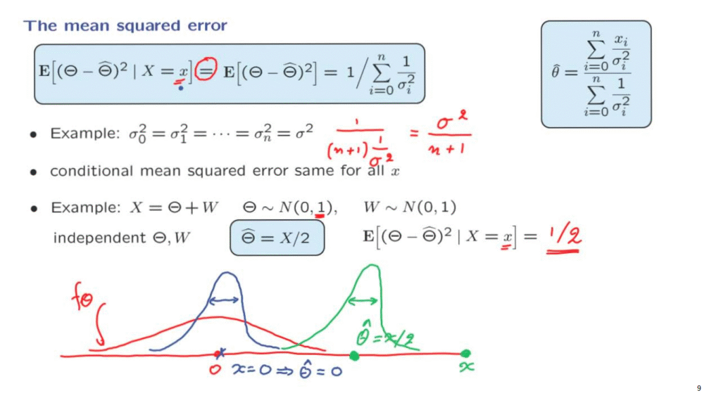
Now, perhaps the most interesting aspect of the facts that we have established is this equation here that tells us that not matter what this value of little x is, the conditional variance, the variance of the posterior distribution of Theta, is going to be the same.
In some sense, it tells us that no particular value of X is more informative or more desirable than any other value.
In order to really appreciate what that statement is really saying, it’s better to look at a very concrete example.
So let us revisit the very first example that we studied, in which case, we only have one observation and where Theta and W are standard normal random variables.
We did go through that example.
And we found that the estimator, the maximum posterior probability estimator, was 1/2 of the observation.
And now we are in a position to also calculate the conditional mean squared error given any particular observation.
We apply this formula.
In fact, we are dealing with this special case with sigma equal to 1.
So we use this expression here.
And we see that it is 1/2.
So we started with a prior variance for Theta, which was 1.
And after we obtained the observation, our uncertainty gets reduced and the variance goes down to 1/2.
And this is true no matter what little x is.
Pictorially, here is what’s happening.
We start with Theta being a standard normal.
So it has a distribution of this form, centered at 0.
This is a plot of the density of Theta, the prior density.
Suppose that we obtain a measurement.
And that measurement happens to be equal to 0.
If the measurement is equal to 0, then our estimate will also be equal to 0.
The posterior distribution of theta is going to be a normal distribution whose mean is the estimate and whose variance is this quantity that we have calculated, which is 1/2.
And therefore, it is narrower than the original PDF that we started from.
So initially, we had a fair amount of uncertainty about Theta.
After we obtained a measurement of 0, this kind of reinforces our belief that Theta is somewhere near 0.
And so we obtain a narrower distribution.
This is our updated belief about Theta.
But what if I happen to obtain a measurement that’s somewhere out here?
In this case, my estimate is going to be 1/2 of what I observed.
It’s here.
And the posterior PDF of Theta is going to be a normal PDF that’s centered around this point and has the same variance, 1/2.
So in some sense, this particular measurement would be thought of as a quite abnormal one.
We’re really surprised to obtain an observation which is so far away from 0.
Because our prior distribution told us that Theta is somewhere here.
So we have been surprised.
But after the surprise and after we form our estimate of Theta, our state of knowledge about Theta is that Theta is a random variable and it has a distribution that’s normal, centered around this point, and whose width is the same no matter what particular observation I happen to get.
So even though this particular observation value is unusual, after it is obtained, the remaining uncertainty about Theta is the same as if we had obtained any other particular value of X.
So this is a very remarkable property that’s special to this type of estimation problems involving normal random variables and linear relations.
It has a very nice side effect.
It means that we can report, we can say anything there is to be said about the performance of this maximum a posteriori probability estimator.
By just giving a single number, we can characterize performance only in terms of this number, as opposed to having to tell what this conditional mean squared error is for the different values of X.