We are now ready to move on to a model which is quite interesting and quite realistic.
This is a model in which we have an unknown parameter modeled as a random variable that we try to estimate.
This is the random variable, Theta.
And we have multiple observations of that random variable.
Each one of those observations is equal to the unknown random variable, plus some additive noise.
This is a model that appears quite often in practice.
It is often the case that we’re trying to estimate a certain quantity, but we can only observe values of that quantity in the presence of noise.
And because of the noise, what we want to do is to try to measure it to multiple times.
And so we have multiple such measurement equations.
And then we want to combine all of the observations together to come up with a good estimate of that parameter.
The assumption that we will be making are that Theta is a normal random variable.
It has a certain mean that we denote by x0.
The reason for this strange notation will be seen later.
And it also has a certain variance.
The noise terms are also normal random variables with 0 mean and a certain variance.

And finally, we assume that these basic random variables that define our model are all independent.
Based on these assumptions, now we would like to estimate Theta on the basis of the X’s.
And as usual, in the Bayesian setting, what we want to do is to calculate the posterior distribution of Theta, given the X’s.
The Bayes rule has the usual form for the case of continuous random variables.
The only remark that needs to be made is that in this case, there are multiple X’s, so X up here stands for the vector of the observations that we have obtained.
And similarly, little x will stand for the vector of the values of these observations.
So we need now to start making some progress towards calculating this term here.
What is the distribution of the vector of measurements given theta.
Before we move to the vector case, let us look at one of the measurements in isolation.
This is something that we have already seen.
If I tell you the value of the random variable, Theta, which is what happens in this conditional universe when you condition on the value of Theta, then in that universe, the random variable, Xi, is equal to the numerical value that you gave me for Theta, plus Wi.
And because Wi is independent from the random variable Theta, knowing the value of the random variable Theta does not change the distribution of Wi.
It will still have this normal distribution.
So Xi is a normal of this kind plus a constant.
And so Xi is a normal random variable with mean equal to the constant that we added, and variance equal to the original variance of the random variable, Wi.
And so we can now write down, the PDF, the conditional PDF, of Xi.
There’s going to be a normalizing constant.
And then the usual exponential term, which is going to be xi minus the mean of the distribution, which is theta.
And then we divide by the usual variance term.
Let us move next to this distribution here.
This is a shorthand notation for the joint PDF of the random variables X1 up to Xn, conditional on the random variable Theta.
So it’s really a function of multiple variables.
And how do we proceed now?
Here is the crucial observation.
If I tell you the value of the random variable capital Theta as before, then you argue as follows.
All of these random variables are independent.
So if I tell you the value of the random variable Theta, this does not change the joint distribution of the Wi’s.
The Wi’s were independent when we started, so they remain independent in the conditional universe.
And since the Wi’s are independent and Xi’s are obtained from the Wi’s by just adding a constant, this means that the Xi’s are also independent in this conditional universe.
Once I tell you the value of Theta, then because the noises are independent, the observations are also independent.
But this means that the joint PDF factors as a product of the individual marginal PDFs of the Xi’s.
And these PDFs, we have already found.
So now, we can put everything together to write down a formula for the posterior PDF using the Bayes rule.
We have this denominator term, which I will write first, and which term we do not need to evaluate.
Then we have the marginal PDF of Theta.
Now since Theta is normal with these parameters, this is of the form e to the minus theta minus x0 squared over 2 sigma 0 squared.
And then we have this joint density of the X’s conditioned on Theta, which we have already found, it is this product here.
It’s a product of n terms, one for each observation.
And each one of these terms is what we have found earlier, so I’m just substituting this expression up here.
Now once we have obtained the observations, so the value of the random variable capital X, that is, the value little x, is fixed.
Once it is fixed, then the x’s that appear here are constant.
So in particular, this term here is a constant.
We do not bother with it.
And what we have is a constant times an exponential in terms that are quadratic in theta.
So we recognize this kind of expression.
It has to correspond to a normal distribution.
And this is the first conclusion of this exercise.
That is, the posterior PDF of the parameter, Theta, given our observations, this posterior PDF is normal.
We have e to a quadratic function in theta.
And that quadratic function also involves the specific values of the X’s that we have obtained.
Let us copy what we have found and rearrange it.
Once more, we have a constant, then the exponential of the negative of some quadratic function in theta.
And the specific quadratic function that we calculated just before takes this particular form.
What is the mean of this normal distribution?
The mean is same as the peak.
And to find the peak, the location at which this PDF is largest, what we do is we try to find the place at which this quadratic function is smallest.
So what we do is to take the derivative with respect to theta of this quadratic, and set it to 0.
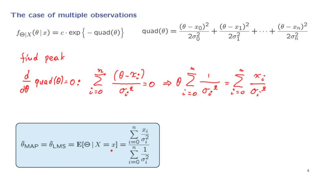
This gives us a sum of terms.
The derivative of the typical term is going to be theta minus xi, divided by sigma i squared.
And this expression must be equal to 0 if theta is at the peak of the posterior distribution.
And so we now rearrange this equation.
We split and take first the term involving theta, and gives us a contribution of this kind.
And we move the terms involving x’s to the other side.
And this gives us this expression.
And finally, we take this sum here and send it to the denominator of the other side.
And this gives us the final form of the solution: the peak of the posterior distribution, which is also the same as the conditional expectation of the posterior distribution.
Whenever we have a normal distribution, the expected value is the same as the place where the distribution is largest.
Let us now conclude with a few comments and words about how to interpret the result that we found.
First, let me emphasize that the same conclusions that we have obtained for the case of a single observation go through in this case as well.
The posterior distribution of the unknown parameter is still a normal distribution.
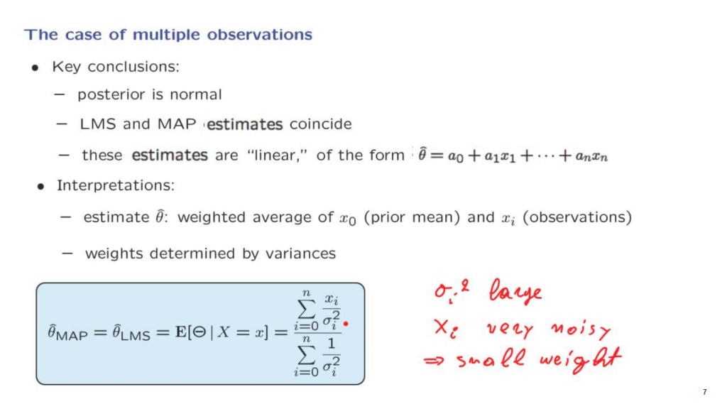
Our state of knowledge about Theta after we obtain the observations is described by a normal distribution.
Because it is a normal distribution, the location of its peak is the same as the expected value.
And for this reason, the conditional expectation estimate and the maximum a posteriori probability estimates coincide.
And finally, the form of the estimates that we get is a linear function in the xi’s.
And this linearity is a very convenient property to have, because it allows further analysis of these ways of obtaining estimates.
How do we interpret this formula?
What we have here is the following.
Each one of the xi’s gets multiplied by a certain coefficient, which is 1 over the variance.
And in the denominator, we have the sum of all of those coefficients.
So what we really have here is a weighted average of the xi’s.
Now keep in mind that those xi’s are not all of them of the same kind.
One term is x0, which is the prior mean, whereas the remaining xi’s are the values of the observations.
So there’s something interesting happening here.
We combine the values of the observations with the value of the prior mean.
And in some sense, the prior mean is treated as just one more piece of information available to us.
And it is treated in a sort of equal way as the other observations.
The weight that we have in this weighted average are that each xi gets divided by the corresponding variance.
Does this make sense?
Well, suppose that sigma i squared is large.
This means that the noise term Wi is very large.
So Xi is very noisy.
And so it’s not a useful observation to have.
And in that case, it gets a small weight.
So the weights are determined by the variances in a way that is quite sensible.
Those observations that will get the most weight will be those observations for which the corresponding noise variance is small.
So the solution to this estimation problem that we just went through has many nice properties.
First, we stay within the world of normal random variables, because even the posterior is normal.
We stay within the world of linear functions of normal random variables, and the form of the formula that we have, itself, has an appealing intuitive content.