Introduction
As a preparation for more complex and more difficult models, we will start by looking at the simplest model that there is, that involves a linear relation and normal random variables.
Model
The specifics of the model are as follows.
There’s an unknown parameter modeled as a random variable, Theta, that we wish to estimate.
What we have in our hands is Theta plus some additive noise, W.
And this sum is our observation, X.
The assumptions that we make are that Theta and W are normal random variables.
And to keep the calculations simple, we assume that they’re standard normal random variables.
Furthermore, we assume that Theta and W are independent of each other.
Inference
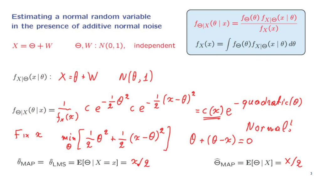
According to the Bayesian program, inference about Theta is essentially the calculation of the posterior distribution of Theta if I tell you that the observation, capital X takes on a specific value little x.
To calculate this posterior distribution, we invoke the appropriate form of the Bayes rule.
We have the prior of Theta.
It’s a standard normal.
Now we need to figure out the conditional distribution of X given Theta.
What is it?
If I tell you that the random variable, capital Theta, takes on a specific value, little theta, then in that conditional universe, our observation is going to be that specific value of Theta, which is our little theta, plus the noise term, capital W.
This is the relation that’s holds in the conditional universe, where we are told the value of Theta.
Now W is independent of Theta.
So even though I have told you the value of Theta, the distribution of W does not change.
It is still a standard normal.
So X is a standard normal plus a constant theta.
What that does is that it changes the mean of the normal distribution, but it will still be a normal random variable.
So in this conditional universe, X is going to be a normal random variable with mean equal to theta, and with variance equal to the variance of W, which is equal to 1.
So now, we know what this distribution is, and we can move with the calculation of the posterior.
So we have the denominator term, which I’m writing here.
And then we have the density of Theta.
Since it is a standard normal, it takes the form of a constant.
We do not really care about the value of that constant.
What we care really is the term on the exponent.
And then we have the conditional density of X given Theta, which is a normal with these parameters.
And therefore, it takes the form c e to the minus 1/2.
It’s a density in x.
And so, up here, we have x minus the mean of that density.
But the mean is equal to theta, squared.
And this is the final form.
Now what we notice here is that we have a few constant terms.
Another term that depends on x, and then a quadratic in theta.
So we can write all this as some function of x, and then e to the negative of some quadratic in theta.
Now when we’re doing inference, we are given the value of X.
So let us fix a particular value of little x and concentrate on the dependence on theta.
So with x being fixed, this is just a constant.
And as a function of theta, it’s e to the minus something quadratic in theta.
And we recognize that this is a normal PDF.
So we conclude that the posterior distribution of Theta, given our observation, is normal.
Since it is normal, the expected value of this conditional PDF will be the same as the peak of that the PDF.
And this would be our point estimate of Theta in particular.
If we use either of the MAP– Maximum A Posterior Probability– or the least mean squares estimator, which is defined as the conditional expectation of Theta, given the observation that we have made.
So this conditional expectation is just the mean of this posterior distribution.
It is also the peak of that posterior distribution.
So let us find what the peak is.
To find the peak, we focus on the exponent term, which is ignoring the minus sign, the exponent term is this one.
And to find the peak of the distribution, we need to find the place where this exponent term is smallest.
To find out when this term is smallest, we take its derivative with respect to theta and set it equal to 0.
The derivative of this term is theta.
The derivative of this term is theta minus x.
We set this to 0.
And when we solve this equation, we find 2 theta equal to x.
Therefore, theta is equal to x/2.
And so, we conclude from here that the peak of the distribution occurs when theta is equal to x/2.
And this is our estimate of theta.
So our estimate takes into account that we believe that theta is 0 on the average.
But also takes into account the observation that we have made, and comes up with a value that’s in between our prior mean, which was 0, and the observation, which is little x.
So this is what the estimates are.
If we want to talk about estimators, which are now random variables, what would they be?
The estimator is a random variable that takes this value whenever capital X takes the value of little x.
Therefore, it’s the random variable, which is equal to capital X/2.
This is a relation between random variables.
This is a corresponding relation between numbers if you’re given a specific value for little x.
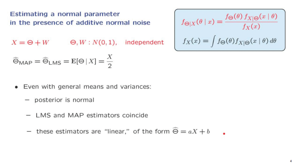
How special is this example?
It turns out that the same structure of the solution shows up even if we assume that Theta and W are independent normal random variables, but with some general means and variances.
You should be able to verify on your own by repeating the calculations that we just carried out that the posterior distribution of Theta will still be normal.
And since it is normal, the peak of the distribution is the same as the expected value.
So the expected value, or least mean squares estimator, coincides with the maximum a-posteriori probability estimator.
And finally, although this formula will not be exactly true, there will be a similar formula for the estimator, namely the estimator will turn out to be a linear function of the measurements.
We will see that these conclusions are actually even more general than that.
And this is what makes it very appealing to work with normal random variables and linear relations.