In this lecture sequence, we will do a lot with normal random variables.
And for this reason, it is useful to start with a simple observation that will allow us later on to move much faster.
Recall that a normal random variable with a certain mean and variance has a PDF of this particular form.
What if somebody gives you a PDF of this form and asks you what it corresponds to?
You can answer that this is exactly of this form provided that you make the identification that 3 is equal to mu.
So this is a normal PDF with a mean equal to 3 and whose variance can also be found by matching this constant that appears here with the number 8.
This constant here is in the denominator.
So we have a term 1/2 sigma squared.
This must be equal to 8.
And from this, we can infer that the variance of this random variable is equal to 1/16.
And if you also want to find out the value of this constant c, you check the formula for normal PDFs, the constant c is 1 over the standard deviation, which is 1/4 in our case.
The square root of this number times the square root of 2 pi.
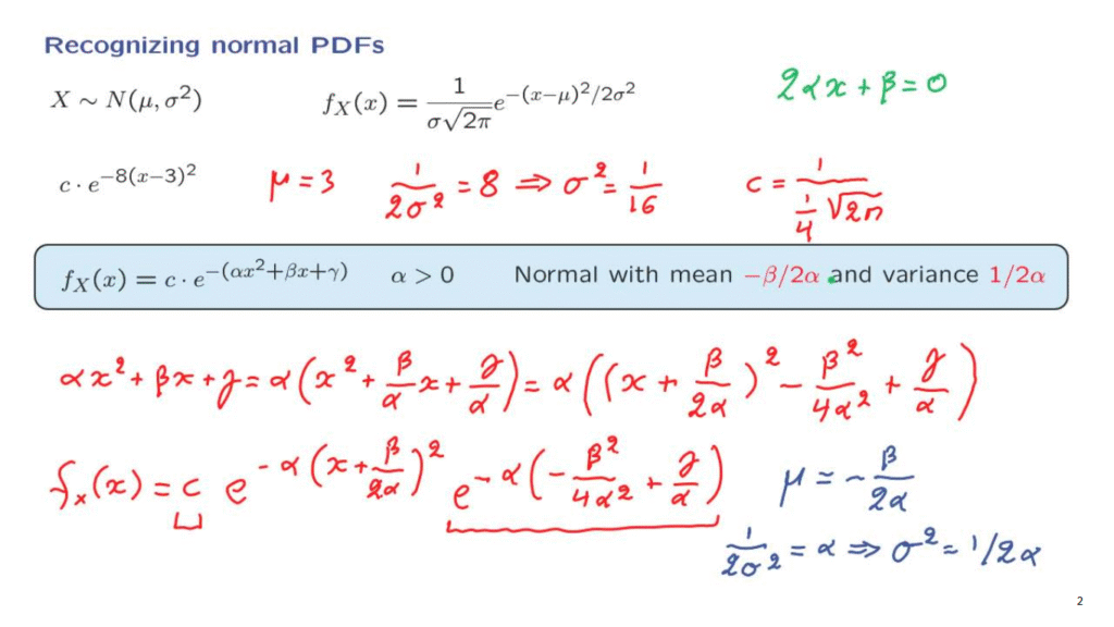
Now suppose that somebody gives you a PDF of this form.
It’s a constant times a negative exponential of a quadratic function in x.
We will argue that this PDF is also a normal PDF.
And identify the parameters of that normal.
First, let’s start with a certain observation.
A PDF must integrate to 1 so it cannot blow up as x goes to infinity, which means that this exponential needs to die out as x goes to infinity.
And that will only happen if this coefficient alpha here is positive.
So that we have e to the minus something positive and large which is going to die out.
Therefore, we must have alpha being a positive constant.
And let us assume from now on that this is the case.
What we will do next is we will try to write this PDF in this form.
And the trick that we’re going to use is the following.
We will focus on the term in the exponent, which we rewrite this way.
We take out a factor of alpha.
And then we will try to make this expression here appear like a square of this kind, like a perfect square.
So what is involved is a certain method, a certain trick called completing the square.
That is, we write this term here in the form x plus something squared.
And then we may need some additional terms.
What should that something be?
We would like that something be such that when we expand this quadratic, we get this term and that term.
Well we get an x squared and then there’s going to be a cross term.
What do we need here so that the cross term is equal to this?
What we need is a term equal to beta over 2 alpha.
Because in that case, the cross term is going to be 2 times x times beta divided by 2 alpha.
The 2 in the beginning and that 2 cancel out, so we’re left with x beta over alpha which is exactly what we got here.
However, this quadratic is going to have an additional term which is going to be the square of this, which is not present here.
So to keep the two sides equal, we need to subtract that term.
And finally, we have the last term involving gamma.
Therefore, the PDF of X is of the form.
We have a certain constant from here.
Then, we have the negative exponential of this term, e to the minus alpha x plus beta over 2 alpha squared.
And then there’s the negative exponential of the rest, which is going to be a term of the form e to the minus alpha times beta squared over 4 alpha squared plus gamma over alpha.
Now this term here does not involve any x’s.
So it can be absorbed into the constant c.
The dependence on x is only through this term.
And now this term looks exactly like what we’ve got up here, provided that you make the following identifications.
Mu has to be equal to what we have here, but here there’s a minus sign, here there’s no minus sign.
And so mu is going to be the negative of what we have up here.
It’s minus beta over 2 alpha.
And as for sigma squared, we match and say that 1/2 sigma squared must be equal to the constant that we have up here, which is alpha.
And from this, we conclude that sigma squared is equal to 1/2 alpha.
So we have concluded that a PDF of this type is indeed a normal PDF.
It has a mean equal to that value.
And a variance equal to that value.
Actually, to figure out what the mean of this PDF is, we do not need to go through this whole exercise.
Once we’re convinced that this is a normal PDF, then we know that the mean is equal to the peak of the PDF.
To find the peak, we want to maximize this over all x’s, which is the same as minimizing this quadratic function over all x’s.
Where is this quadratic function minimized?
To find that place, we can look at the exponent, take its derivative, and set it to 0.
So setting the derivative of the exponent to 0 gives us the equation 2 alpha x plus beta equal to 0.
And from this, we solve for x.
And we can tell that the peak of the distribution is going to be when x takes this particular value.
This value must also be equal to the mean.
So this is a very useful fact to know.
And we will use it over and over.
Negative exponential of a quadratic function of x is always a normal PDF.