We will now go through an example that involves a continuous unknown parameter, the unknown bias of a coin and discrete observations, namely, the number of heads that are observed in a sequence of coin flips.
This is an example that we will start in some detail now, and we will also revisit later on.
And in the process, we will also have the opportunity to introduce a new class of probability distributions.
This example is an extension of an example that we have already seen, when we first introduced the relevant version of the Bayes rule.
We have a coin.
It has a certain bias between 0 and 1, but the bias is unknown.
And consistent with the Bayesian philosophy, we treat this unknown bias as a random variable, and we assign a prior probability distribution to it.
We flip this coin n times independently, where n is some positive integer, and we record the number of heads that are obtained.
On the basis of the value of this random variable, we would like to make inferences about Theta.
Now to make some more concrete progress, let us make a specific assumption.
Let us assume that the prior on Theta is uniform on the unit interval, in some sense reflecting complete ignorance about the true value of Theta.
We observe the value of this random variable, some little k, we fix that value, and we’re interested in the functional dependence on theta of this particular quantity, when k is given to us.
How do we do this?
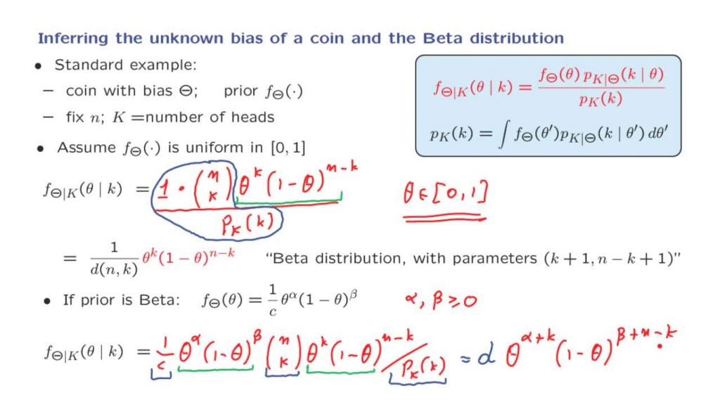
We use the appropriate form of the Bayes rule, which in this setting is as follows.
it is the usual form, but we have f’s indicating densities whenever we’re talking about the distribution of Theta, because Theta is continuous.
And whenever we talk about the distribution of K, which is discrete, we use the symbol p, because we’re dealing with probability mass functions.
As always, the denominator term is such that the integral of the whole expression over theta is equal to 1.
This is the necessary normalization property, and because of this, this denominator term has to be equal to the integral of the numerator over all theta, which is what we have here.
So now let us move, and let us apply this formula.
We first have the prior, which is equal to 1.
Then we have the probability that K is equal to little k.
This is the probability of obtaining exactly k heads, if I tell you the bias or the coin.
But if I tell you the bias of the coin, we’re dealing with the usual model of independent coin flips, and the probability of k heads is given by the binomial probabilities, which takes this form.
And finally, we have the denominator term, which we do not need to evaluate at this point.
Now, I said earlier that we’re interested in the dependence on theta, which comes through these terms.
On the other hand, the remaining terms do not involve any thetas, and so they can be lumped together in just a constant.
And so we can write the answer that we have found in this more suggestive form.
We have some normalizing constant, and here we keep separately the dependence on theta.
Of course, this answer that we derived is valid for little theta belonging to the unit interval.
Outside the unit interval, either the prior density or the posterior density of Theta would be equal to 0.
This particular form of the posterior distribution for Theta is a certain type of density, and it shows up in various contexts.
And for this reason, it has a name.
It is called a Beta distribution with certain parameters, and the parameters reflect the exponents that we have up here in the two terms.
Note that these parameters are the exponents augmented by 1.
This is for historical reasons that do not concern us here.
It is just a convention.
The important thing is to be able to recognize what it takes for a distribution to be a Beta distribution.
That this that the dependence on theta is of the form theta to some power times 1 minus theta to some other power.
Any distribution of this form is called a Beta distribution.
So now, let’s continue this example by considering a different prior.
Suppose that the prior is itself a Beta distribution of this form where alpha and beta are some non-negative numbers.
What is the posterior in this case?
We just go through the same calculation as before, but instead of using one in the place of the prior, we now use the prior that’s given to us.
The probability of k heads in the n tosses, when we know the bias, is exactly as before.
It is given by the binomial probabilities.
And finally, we need to divide by the denominator term, which is the normalizing constant.
What do we observe here?
The dependence on theta comes through these terms.
The remaining terms do not involve theta, and they can all be absorbed in a constant.
Let’s call that constant d, and collect the remaining terms.
We have theta to the power of alpha plus k, and then, 1 minus theta to the power of beta plus n minus k.
And once more, this is the form of the posterior for thetas belonging to this range.
The posterior is 0 outside this range.
So what do we see?
We started with a prior that came from the Beta family of this form, and we came up with a posterior that is still a function of theta of this form, but with different values of the parameters alpha and beta.
Namely, alpha gets replaced by alpha plus k, beta gets replaced by beta plus n minus k.
So we see that if we start with a prior from the family of Beta distributions, the posterior will also be in that same family.
This is a beautiful property of Beta distributions that can be exploited in various ways.
One of which is that it actually allows for recursive ways of updating the posterior of Theta as we get more and more observations.