In the next variation we consider, all random variables are continuous.
For this case, we do have a Bayes rule, once more.
And we have worked [out] quite a few examples.
So there’s no point, again, in going through a detailed example.
Let us just discuss some of the issues.
One question is when do these models arise?
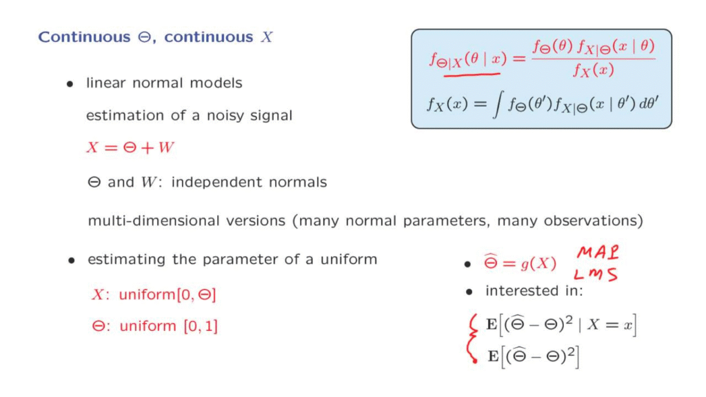
One particular class of models that is very useful and very commonly used are so-called linear normal models.
In these models, we, basically, combine various random variables in a linear function.
And all the random variables of interest are now to be normal.
For instance, we might have a signal, a noisy signal, call it Theta, which is now a continuous valued signal.
We receive that signal, but corrupted by some noise, which is independent from what was sent.
And we wish to recover, on the basis of the observation X, we wish to recover the value of Theta.
And then there are versions of this problem that involve Theta vectors instead of single values.
So that Theta consists of multiple components, and where we obtain many measurements X.
We will, actually, see in the next lecture sequence, a quite detailed discussion of models of this type.
And this will be one of our main examples within our study of inference.
There will be another example that we will see a few times, and this involves estimating the parameter of a uniform distribution.
So X is a random variable that’s uniform over a certain range.
But the range itself is random and unknown.
And on the basis of observations X, we would like to make an estimation of what the true value of Theta is.
This is an example that you will see in our collection of solved problems for this class.
So what are the questions in this setting, we wish to come up with ways of estimating Theta, we form an estimator, and the main candidates for estimators at this points are, once more, the maximum a posteriori probability estimator, which looks at this conditional density and picks a value of theta that makes this conditional density as large as possible.
And then the alternative one is the least mean squares estimator, which just computes the expected value of Theta given X.
For any given estimator, we then want to characterize its performance.
In this case, a natural notion of performance is the distance between our estimate, or estimator, from the true value of Theta.
And commonly we use the squared distance and then take the average of that squared distance.
So in a conditional universe where we have already observed some data, we might be interested in this particular expectation, which is the mean squared error of this particular estimator, given that we obtain some particular data.
Or we can average over all possible data points that we might obtain so that we look at the unconditional mean squared error, which is a measure of the overall performance of our estimator.
We will be talking about these criteria and the mean squared error in a fair amount of detail in a subsequent lecture sequence.