In the next variation that we consider, the random variable Theta is still discrete.
So it might, for example, represent a number of alternative hypothesis.
But now our observation is continuous.
Of course, we do have a variation of the Bayes rule that’s applicable to this situation.
The only difference from the previous version of the Bayes rule is that now the PMF of X, the unconditional and the conditional one, is replaced by a PDF.
Otherwise, everything remains the same.
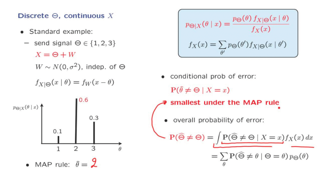
A standard example is the following.
Here we’re sending a signal that takes one of, let’s say, three alternative values.
And what we observe is the signal that was sent plus some noise.
And the typical assumption here might be that the noise has zero mean and a certain variance, and is independent from the signal that was sent.
This is an example that we more or less studied some time ago.
Actually, at that time, we looked at an example where Theta could only take one out of two values, but the calculations and the methodology remains essentially the same as for the case of three values.
So in principle, we do know at this point how to apply the Bayes rule in this situation to come up with a conditional PMF of theta.
And the key to that calculation was that the term that we need, the conditional PDF of X, can be obtained from this equation as follows.
If I tell you the value of Theta, then X is essentially the same as W plus a certain constant.
Adding a constant just shifts the PDF of W by an amount equal to that constant.
And, therefore, the conditional PDF of X is the shifted PDF of the random variable W.
Using this particular fact, we can then apply the Bayes rule, carry out of the calculations, and suppose that in the end we came up with these results.
That is we obtain the specific observation x and based on that observation, we calculate the conditional probabilities of the different choices of Theta.
At this point, we may use the MAP rule and come up with an estimate which is the value of Theta, which is the more likely one.
And then we can continue exactly as in the case of discrete measurements, of discrete observations, and talk about conditional probabilities of error and so on.
Now, the fact that X is continuous really makes no difference, once we arrive at this picture.
With the MAP rule we still choose the most likely value of theta, and this is our estimates.
And we can calculate the probability of error, which with the MAP rule would be 0.
4, exactly the same argument as for the case of discrete observations applies and shows that this conditional probability of error is smallest under the MAP rule.
And then we can continue similarly and talk about the overall probability of error, which can be calculated using the total probability theorem in two ways.
One way is to take the conditional probability of error for any given value of X and then average those conditional probabilities of errors over all the possible choices of X.
Because X is now continuous, here we’re going to have an integral.
Alternatively, you can condition on the possible values of Theta, calculate conditional probabilities of error for any particular choice of theta, and then take a weighted average of them.
In practice, this calculation sometimes turns out to be the simpler one.
Finally, we can replicate the argument that we had in the discrete case.
Since the MAP rule makes this term here as small as possible, it is less than or equal to the probability of error that you would get under any other estimate or estimator, then it follows that the integral will also be as small as possible.
And therefore, the conclusion is that the overall probability of error is, again, the smallest possible when we use the MAP rule.
And so the MAP rule remains the optimal way of choosing between alternative hypothesis, whether X is discrete or continuous.