Let us now discuss in some more detail what it takes to carry out Bayesian inference, when both random variables are discrete.
The unknown parameter, Theta, is a random variable that takes values in the discrete set.
And we can think of these values as alternative hypotheses.
In this case, we know how to do inference.
We have in our hands the Bayes rule and we have seen plenty of examples.
So instead of going through one more example in detail, let us assume that we have a model, that we have observed the value of X, and that we have already determined the conditional PMF of the random variable Theta.
As a concrete example, suppose that Theta can take values 1, 2, or 3.
We have obtained our observation, and the conditional PMF takes this form.
We could stop at this point or we could continue by asking for a specific estimate of Theta– our best guess as to what Theta is.
One way of coming up with an estimate is to use the maximum a posteriori of probability rule, which looks for that value of theta that has the largest posterior, or conditional, probability.
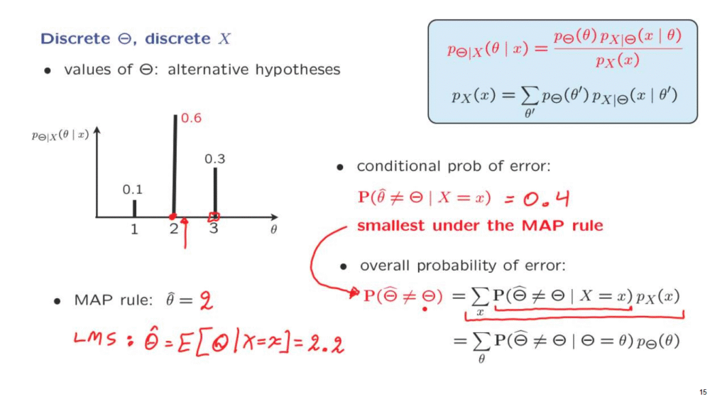
In this example, it is this value, so our estimate is going to be equal to 2.
An alternative way of coming up with an estimate could be the LMS rule, which calculates an estimate equal to the conditional expectation of the unknown parameter, given the observation that we have made.
This is just the mean of this conditional distribution.
In this example, it would fall somewhere around here, and the numerical value, as you can check, is equal to 2.2.
Next, we may be interested in how good a certain estimate is.
And for the case where we interpret the values of Theta as hypotheses, a relevant criterion is the probability of error.
In this case, because we already have some data available in our hands and we’re called to make an estimate, what we care about is the conditional probability, given the information that we have, that we’re making an error.
Making an error means the following.
We have the observation, the value of the estimate has been determined, it is now a number, and that’s why we write it with a lowercase theta hat.
But the parameter is still unknown.
We don’t know what it is.
It is described by this distribution.
And there’s a probability that it’s going to be different from our estimate.
What is this probability?
It depends on how we construct the estimates.
If in this example, we use the MAP rule and we make an estimate of 2, there is probability 0.6 that the true value of Theta is also equal to 2, and we are fine.
But there’s a remaining probability of 0.4 that the true value of Theta is different than our estimate.
So there’s probability 0.4 of having made a mistake.
If, instead of an estimate equal to 2, we had chosen an estimate equal to 3, then the true parameter would be equal to our estimate with probability 0.3, but we would have made an error with probability 0.7, which would be a bigger probability of error.
More generally, the probability of error of a particular estimate is the sum of the probabilities of the other values of Theta.
And if we want to keep the probability of error small, we want to keep the sum of the probabilities of the other values small, which means we want to pick an estimate for which its own probability is large.
And so by that argument, we see that the way to achieve the smallest possible probability of error is to employ the MAP rule.
This is a very important property of the MAP rule.
Now, this is the conditional probability of error, given that we already have data in our hands.
But more generally, we may want to compare estimators or talk about their performance in terms of their overall probability of error.
We’re designing a decision-making system that’s going to process data and making decisions.
In order to say how good our system is, we want to say that overall, whenever you use the system, there’s going to be some random parameter, there’s going to be some value of the estimate.
And we want to know what’s the probability that these two will be different.
We can calculate this overall probability of error by using the total probability theorem.
And the conditional probabilities of error as follows.
We condition on the value of X.
For any possible value of X, we have a conditional probability of error.
And then we take a weighted average of these conditional probabilities of error.
There’s also an alternative way of using the total probability theorem, which would be to first condition on Theta and calculate the conditional probability of error for a given choice of this unknown parameter.
And both of these formulas can be used.
Which one of the two is more convenient really depends on the specifics of the problem.
Finally, I would like to make an important observation.
We argued that for any particular choice of an observation, the MAP rule achieves the smallest possible probability of error.
So under the MAP rule, this term is as small as possible for any given value of the random variable, capital X.
Since each term of this sum is as small as possible under the MAP rule, it means that the overall sum will also be as small as possible.
And this means is that the overall probability of error is also smallest under the MAP rule.
In this sense, the MAP rule is the optimum way of coming up with estimates in the hypothesis-testing context, where we want to minimize the probability of error.