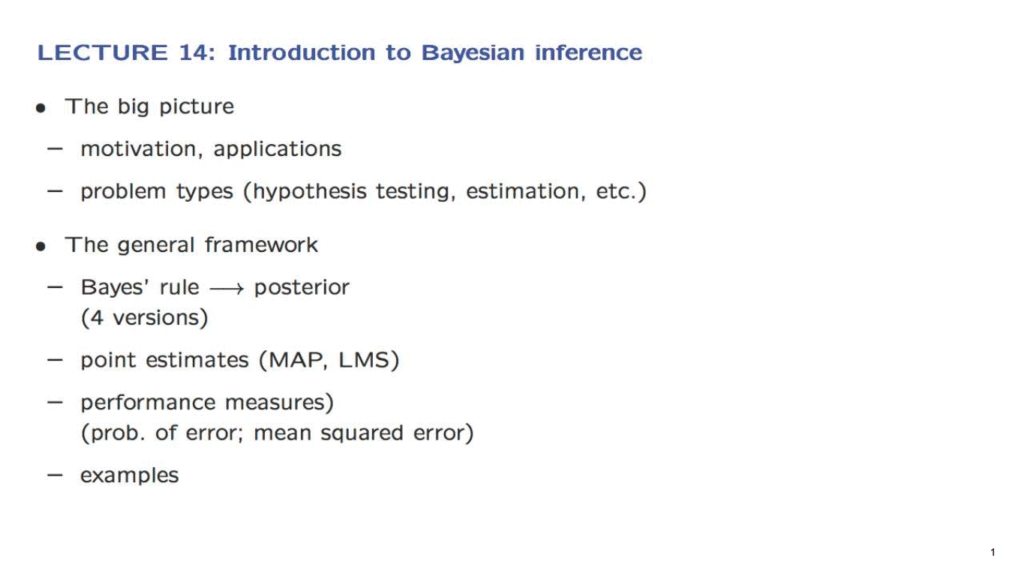
In this lecture, we start our systematic study of Bayesian inference.
We will first talk a little bit about the big picture, about inference in general, the huge range of possible applications, and the different types of problems that one may encounter.
For example, we have hypothesis testing problems in which we are trying to choose between a finite and usually small number of alternative hypotheses or estimation problems where we want to estimate as close as we can an unknown numerical quantity.
We then move into the specifics of Bayesian inference.
The central idea is that we always use the Bayes rule to find the posterior distribution of an unknown random variable based on observations of a related random variable.
Depending on whether the random variables are discrete or continuous, we must of course you use the appropriate version of the Bayes rule.

If we want to summarize the posterior in a single number, that is, to come up with a numerical estimate of the unknown random variable, we then have some options.
One is to report the value at which the posterior is largest.
Another is to report the mean of the conditional distribution.
These go under the acronyms MAP and LMS.
We will see shortly what these acronyms stand for.
Given any particular method for coming up with a point estimate, there are certain performance metrics that tell us how good the estimate is.
For hypothesis testing problems, the appropriate metric is the probability of error, the probability of making a mistake.
For problems of estimating a numerical quantity, an appropriate metric that we will be using a lot is the expected value of the squared error.
As we will see, there will be no new mathematics in this lecture, just a few definitions, a few new terms, and an application of the Bayes rule.
Nevertheless, it is important to be able to apply the Bayes rule systematically and with confidence.
For this reason, we will be going over several examples.