This is an example, or rather, a story, that’s supposed to give us some insight and some intuition about what the law of iterated expectations really means.
Suppose that you work for a forecasting company.
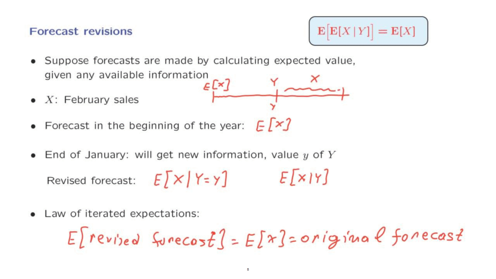
And suppose that you make forecasts by calculating expected values of the quantities that you want to forecast.
And of course, when you calculate an expected value, you always use whatever information you have.
So here we have the beginning of the year.
And you’re working for a company that’s trying to forecast the sales during the month of February.
That’s a random variable, capital X.
You’re sitting in your office in the beginning of the year.
What is going to be your forecast?
It’s going to be the expected value of the random variable X.
So this is a forecast that you make at this point in time.
Now, time goes by, and we’re sitting now in the beginning of February or the end of January.
At that time, you obtain some new information, which is the value, little y, of a random variable, capital Y.
What should your new forecast be?
Well, once you have this information in your hands, your new forecast should be the expected value of x, given the specific available information that you have.
So this is the revised forecast as calculated at the end of January.
But if you’re sitting here in the beginning of the year and you ask yourself, what is the revised forecast going to be, your answer would be, I don’t know what it’s going to be.
It’s random.
It depends on what capital Y would end up being.
My revised forecast is a random variable, the expected value of X given Y, which will take this particular numerical value if it turns out the random variable Y takes a specific value, little y.
So this is the forecast calculated at this point in time.
This is the forecast viewed at the beginning of the year, at which time we do not know yet the value of the revised forecast.
Now, what does the law of iterated expectations tell us in this case?
It tells us that the expected value of the revised forecast is the same as the original forecast.
What does this mean in practical terms?
It means that given today’s forecast, the original forecast, you do not expect the next forecast, the revised one, to be higher or lower.
It could be either higher or lower.
But on the average, you expect the revision of the forecast going from this one to that one, the revised one, that revision on the average, to be equal to 0.
You do not expect forecasts to be revised either upwards or downwards on the average.
Of course, this is not what happens always in real life.
So suppose that capital X, the quantity you’re forecasting, is the cost of some big project.
And your original budget or original forecast, expected value of X, is what you expect the cost of the project to be.
Well, from experience with real life, we kind of know that budgets or cost estimates tend to be revised upwards more often than downwards.
Does this real life fact contradict the law of iterated expectations?
Well, not really.
What is going on here is that real life forecasts are not really honestly calculated expected values.
But maybe they’re calculated with some implicit or hidden biases so that the forecasts that are given are actually not the expected values.
So there’s no contradiction between this mathematical fact and possible life experiences.