We have previously defined the abstract conditional expectation of one random variable given another random variable.
And we discussed that it is, by itself, a random variable.
In particular, it has an expectation, or mean, of its own.
What is this mean?
This is what we want to find out.
Let us recall our development.
We look at the conditional expectation of a random variable given a specific numerical value of another random variable.
This is a number that depends on little y.
And this can be used to define a function little g.
The function little g for any particular little y tells us the numerical value of the conditional expectation.
Since little g is a well defined function, we can also now define this particular function, which is now a function of a random variable.
It’s a well defined object.
It’s a random variable.
And then we introduced this abstract notation.
We defined this object to be exactly this particular random variable.
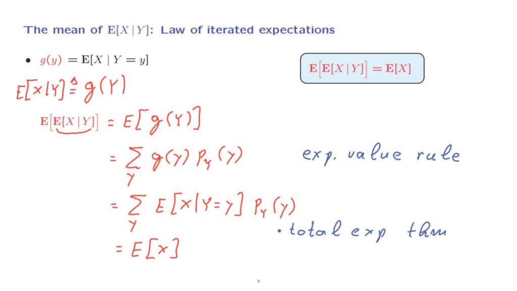
So now we want to calculate the expected value of this object, which is written this way.
Now this notation, here, may look quite formidable, but let’s see what is happening.
Inside here, we have a random variable.
And we take the expected value of that random variable.
Or, more crisply, think of that as the expected value of g of capital Y, where g of capital Y is defined through these correspondences here.
How do we calculate the expected value of a function of a random variable?
Here we use the Expected Value Rule.
Assuming that Y is a discrete random variable, the Expected Value Rule takes this form.
And the next step is to substitute the particular form for g of Y that we have.
g of Y was defined in this manner.
So we’re dealing with the sum over all little y’s of the expected value of X, given that Y takes the value little y, weighted by the PMF of little y.
Now if we look at this expression, then it should look familiar.
It is the expression that appears in the Total Expectation Theorem.
We take the conditional expectation under different scenarios and weigh those conditional expectations according to the probabilities of those scenarios.
And this just gives us the overall expectation of the random variable X.
So this step, here, was carried out using the Total Expectation Theorem.
So we have proved this important fact, that the expectation of a conditional expectation is the same as the unconditional expectation.
This important fact is called the Law of Iterated Expectations.
The proof was carried out assuming that Y is discrete.
So we use this particular version involving a PMF, but the proof is exactly the same for the continuous case.
You would be using an integral and the PDF, instead the PMF.
As the proof indicates, the Law of Iterated Expectations is nothing but an abstract version of the Total Expectation Theorem.
It is really the Total Expectation Theorem written in more abstract notation.
But this turns out to be powerful and also we avoid having to deal separately with discrete or continuous random variables.