Conditional PDFs share most of the properties of conditional PMFs.
All facts for the discrete case have continuous analogs.
The intuition is more or less the same, although it is much easier to grasp in the discrete case.
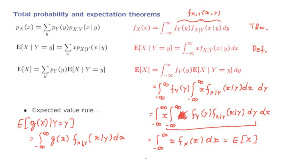
For example, we have seen this version of the total probability theorem.
There is a continuous analog in which we replace sums by integrals.
And we replace PMFs by PDFs.
The proof of this fact is actually pretty simple.
By the multiplication rule, the integrand, here, is just the joint PDF of X and Y.
And we know that if we take the joint PDF and integrate with respect to one variable then we recover the marginal PDF of the other random variable.
So this is one theorem that extends to the continuous case.
Moving along, we have defined the conditional expectation in this manner in the discrete case.
And we define it similarly for the continuous case.
So actually here we now have a new definition.
This definition is also consistent with the definition of the expectation of a continuous random variable.
The expected value for continuous random variable is the integral of X times [a] density.
Except that here we live in a conditional universe where we’re conditioning on this event.
And therefore, we need to use the corresponding conditional PDF.
Finally, we have the total expectation theorem in the discrete case.
And there is the obvious analog in the continuous case where we are using an integral and a density.
The interpretation is that we consider all possibilities for Y.
Under each possibility of Y we find the expected value of X.
And then we weigh those different possibilities according to the corresponding values of the density.
So we’re taking a weighted average of these conditional expectations to obtain the overall expectation of the random variable X.
The derivation of this fact is maybe a little instructive because it uses various facts that we have in our hands.
So let’s see how to derive it.
We start from this expression in the right-hand side and we will show that it is equal to the expected value of X.
The expression on the right-hand side is equal to the following, it’s the integral of the density of Y.
And then, inside here, we have the conditional expectation which is defined this way.
So we just plug-in the definition.
And then what we do, is we take this term and move it inside the integral.
Which we can do because this integral is with respect to x.
And therefore, this is like a constant.
And we also interchange the order of integration.
Now, the inner integration is with respect to y.
As far as Y is concerned, this term, x, is a constant.
So we can take it and move it outside this first integral and place it out there.
So this term disappears and goes out there.
What do we have here? This part, by the previous fact, the total probability theorem, is just the density of X.
So we’re left with the integral of x times the density of x dx.
And this is the expected value of X.
Finally, we have various forms of the expected value rule, which barely deserve writing down.
Because they’re exactly what you might expect.
Consider, for example, an expression such as this one, the expected value of a function of the random variable X but conditioned on the value of the random variable Y.
How do we calculate this quantity? Well, the expected value rule tells us that we should integrate g of x times the density of X.
But because, here we live in a conditional universe, we should actually use the corresponding conditional PDF of X.
And there are many other versions of the expected value rule.
Any version that we have seen for the discrete case has, also, a continuous analog which looks about the same except that we integrate and that we use densities.