In this segment, we start a discussion of multiple continuous random variables.
Here are some objects that we’re already familiar with.
But exactly as in the discrete case, if we are dealing with two random variables, it is not enough to know their individual PDFs.
We also need to model the relation between the two random variables, and this is done through a joint PDF, which is the continuous analog of the joint PMF.
We will use this notation to indicate joint PDFs where we use f to indicate that we’re dealing with a density.
So what remains to be done is to actually define this object and see how we use it.
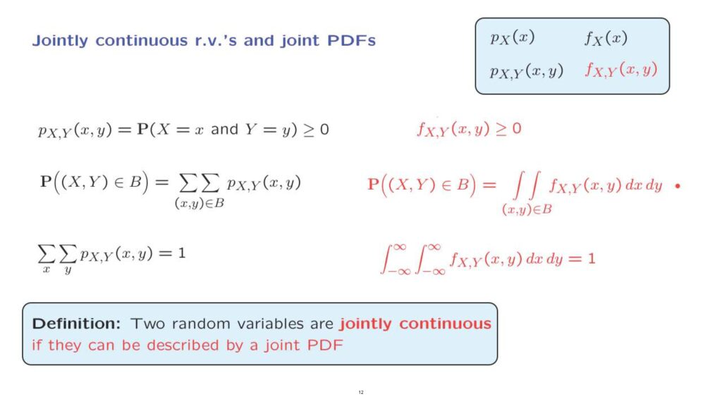
Let us start by recalling that joint PMFs were defined in terms of the probability that the pair of random variables X and Y take certain specific values little x and little y.
Regarding joint PDFs, we start by saying that it has to be non-negative.
However, a more precise interpretation in terms of probabilities has to wait a little bit.
Joint PDFs will be used to calculate probabilities.
And this will be done in analogy with the discrete setting.
In the discrete setting, the probability that the pair of random variables falls inside a certain set is just the sum of the probabilities of all of the possible pairs inside that particular set.
For the continuous case, we introduce an analogous formula.
We use the joint density instead of the joint PMF.
And instead of having a summation, we now integrate.
As in the discrete setting, we have one total unit of probability.
The joint PDF tells us how this unit of probability is spread over the entire continuous two-dimensional plane.
And we use it, we use the joint PDF, to calculate the probability of a certain set by finding the volume under the joint PDF that lies on top of that set.
This is what this integral really represents.
We integrate over a particular two-dimensional set, and we take this value that we integrate.
And we can think of this as the height of an object that’s sitting on top of that set.
Now, this relation here, this calculation of probabilities, is not something that we are supposed to prove.
This is, rather, the definition of what a joint PDF does.
A legitimate joint PDF is any function of two variables, which is non-negative and which integrates to 1.
And we will say that two random variables are jointly continuous if there is a legitimate joint PDF that can be used to calculate the associated probabilities through this particular formula.
So we have really an indirect definition.
Instead of defining the joint PDF as a probability, we actually define it indirectly by saying what it does, how it will be used to calculate probabilities.
A picture will be helpful here.
Here’s a plot of a possible joint PDF.
These are the x and y-axes.
And the function being plotted is the joint PDF of these two random variables.
This joint PDF is higher at some places and lower at others, indicating that certain regions of the x,y plane are more likely than others.
The joint PDF determines the probability of a set B by integrating over that set B.
Let’s say it’s this set.
Integrating the PDF over that set.
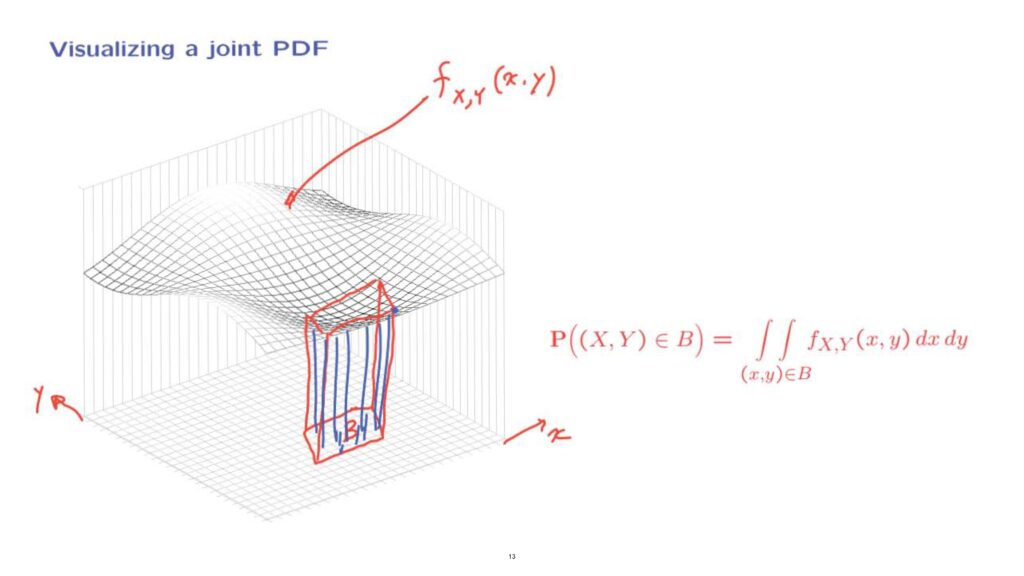
Pictorially, what this means is that we look at the volume that sits on top of that set, but below the PDF, below the joint PDF, and so we obtain some three-dimensional object of this kind.
And this integral corresponds to actually finding this volume here, the volume that sits on top of the set B but which is below the joint PDF.
Let us now develop some additional understanding of joint PDFs.
As we just discussed, for any given set B, we can integrate the joint PDF over that set.
And this will give us the probability of that particular set.
Of particular interest is the case where we’re dealing with a set which is a rectangle, in which case the situation is a little simpler.
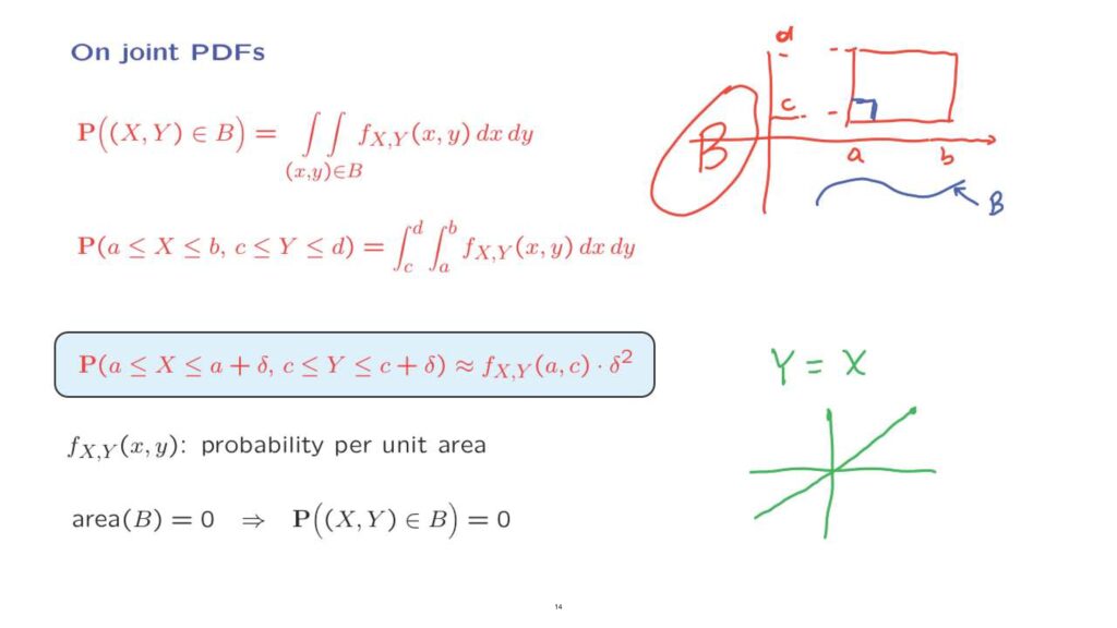
So suppose that we have a rectangle where the x-coordinate ranges from A to B and the y-coordinate ranges from some C to some D.
Then, the double integral over this particular rectangle can be written in a form where we first integrate with respect to one of the variables that ranges from A to B.
And then, we integrate over all possible values of y as they range from C to D.
Of particular interest is the special case where we’re dealing with a small rectangle such as this one.
A rectangle with sizes equal to some delta where delta is a small number.
In that case, the double integral, which is the volume on top of that rectangle, is simpler to evaluate.
It is equal to the value of the function that we’re integrating at some point in the rectangle — let’s take that corner — times the area of that little rectangle, which is equal to delta square.
So we have an interpretation of the joint PDF in terms of probabilities of small rectangles.
Joint PDFs are not probabilities.
But rather, they are probability densities.
They tell us the probability per unit area.
And one more important comment.
For the case of a single continuous random variable, we know that any single point has 0 probability.
This is again, true for the case of two jointly continuous random variables.
But more is true.
If you take a set B that has 0 area.
For example, a certain curve.
Suppose that this curve is the entire set B.
Then, the volume under the joint PDF that’s sitting on top of that curve is going to be equal to 0.
So 0 area sets have 0 probability.
And this is one of the characteristic features of jointly continuous random variables.
Now, let’s think of a particular situation.
Suppose that X is a continuous random variable, and let Y be another random variable, which is identically equal to X.
Since X is a continuous random variable, Y is also a continuous random variable.
However, in this situation, we are certain that the outcome of the experiment is going to fall on the line where x equals y.
All the probability lies on top of a line, and a line has 0 area.
So we have positive probability on the set of 0 area, which contradicts what we discussed before.
Well, this simply means that X and Y are not jointly continuous.
Each one of them is continuous, but together they’re not jointly continuous.
Essentially, joint continuity is something more than requiring each random variable to be continuous by itself.
For joint continuity, we want the probability to be really spread over two dimensions.
Probability is not allowed to be concentrated on a one-dimensional set.
On the other hand, in this example, the probability is concentrated on a one-dimensional set.
And we do not have joint continuity.