We now continue with the development of continuous analogs of everything we know for the discrete case.
We have already seen a few versions of the total probability theorem, one version for events and one version for PMFs.
Let us now develop a continuous analog.
Suppose, as always, that we have a partition of the sample space into a number of disjoint scenarios.
Three scenarios in this picture.
More generally, n scenarios in these formulas.
Let X be a continuous random variable and let us take B to be the event that the random variable takes a value less than or equal to some little x.
By the total probability theorem, this is the probability of the first scenario times the conditional probability of this event given that the first scenario has materialized, and then we have similar terms for the other scenarios.
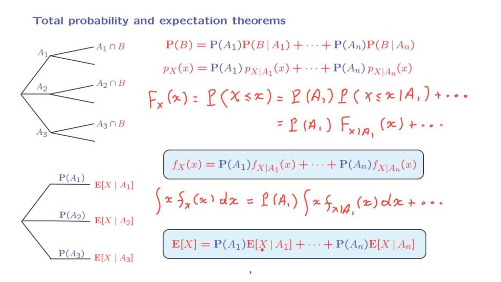
Let us now turn this equation into CDF notation.
The left-hand side is what we have defined as the CDF of the random variable x.
On the right-hand side, what we have is the probability of the first scenario multiplied, again, by a CDF of the random variable X.
But it is a CDF that applies in a conditional model where event A1 has occurred.
And so we use this notation to denote the conditional CDF, the CDF that applies to the conditional universe.
And then we have similar terms for the other scenarios.
Now, we know that the derivative of a CDF is a PDF.
We also know that any general fact, such as this one that applies to unconditional models will also apply without change to a conditional model, because a conditional model is just like any other ordinary probability model.
So let us now take derivatives of both sides of this equation.
On the left-hand side, we have the derivative of a CDF, which is a PDF.
And on the right-hand side, we have the probability of the first scenario, and then the derivative of the conditional CDF, which has to be the same as the conditional PDF.
So we use here the fact that derivatives of CDFs are PDFs, and then we have similar terms under the different scenarios.
So we now have a relation between densities.
To interpret this relation, we think as follows.
The probability of falling inside the little interval around x is determined by the probability of falling inside that little interval under each one of the different scenarios and where each scenario is weighted by the corresponding probability.
Now, we multiply both sides of this equation by x, and then integrate over all x’s.
We do this on the left-hand side.
And similarly, on the right-hand side to obtain a term of this form.
And we have similar terms corresponding to the other scenarios.
What do we have here? On the left-hand side, we have the expected value of x.
On the right-hand side, we have this probability multiplied by the conditional expectation of X given that scenario A1 has occurred.
And so we obtain a version of the total expectation theorem.
It’s exactly the same formula as we had in the discrete case, except that now X is a continuous random variable.
Let us now look at a simple example that involves a model with different scenarios.
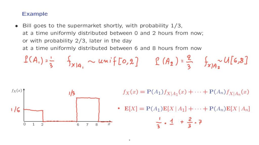
Bill wakes up in the morning and wants to go to the supermarket.
There are two scenarios.
With probability one third, a first scenario occurs.
And under that scenario, Bill will go at a time that’s uniformly distributed between 0 and 2 hours from now.
So the conditional PDF of X, in this case, is uniform on the interval from 0 to 2.
There’s a second scenario that Bill will take long nap and will go later in the day.
That scenario has a probability of 2/3.
And under that case, the conditional PDF of X is going to be uniform on the range between 6 and 8.
By the total probability theorem for densities, the density of X, of the random variable– the time at which he goes to the supermarket– consists of two pieces.
One piece is a uniform between 0 and 2.
This uniform ordinarily would have a height or 1/2.
On the other hand, it gets weighted by the corresponding probability, which is 1/3.
So we obtain a piece here that has a height of 1/6.
Under the alternative scenario, the conditional density is a uniform on the interval between 6 and 8.
This uniform has a height of 1/2 again, but it gets multiplied by a factor of 2/3.
And this results in a height for this term that we have here, which is 1/3.
And this is the form of the PDF of the time at which Bill will go to the supermarket.
We can now finally use the total expectation theorem.
The conditional expectation under the two scenarios can be found as follows.
Under one scenario, we have a uniform between 0 and 2.
And so the conditional expectation is 1, and it gets weighted by the corresponding probability, which is 1/3.
Under the second scenario, which has probability 2/3, the conditional expectation is the midpoint of this uniform, which is 7.
And this gives us the expected value of the time at which he goes.
So this is a simple example, but it illustrates nicely how we can construct a model that involves a number of different scenarios.
And by knowing the probability distribution under each one of the scenarios, we can find the probability distribution overall.
And we can also find the expected value for the overall experiment.