We now introduce normal random variables, which are also often called Gaussian random variables.
Normal random variables are perhaps the most important ones in probability theory.
They play a key role in the theory of the subject, as we will see later in this class in the context of the central limit theorem.
They’re also prevalent in applications for two reasons.
They have some nice analytical properties, and they’re are also the most common model of random noise.
In general, they are a good model of noise or randomness whenever that noise is due to the addition of many small independent noise terms, and this is a very common situation in the real world.
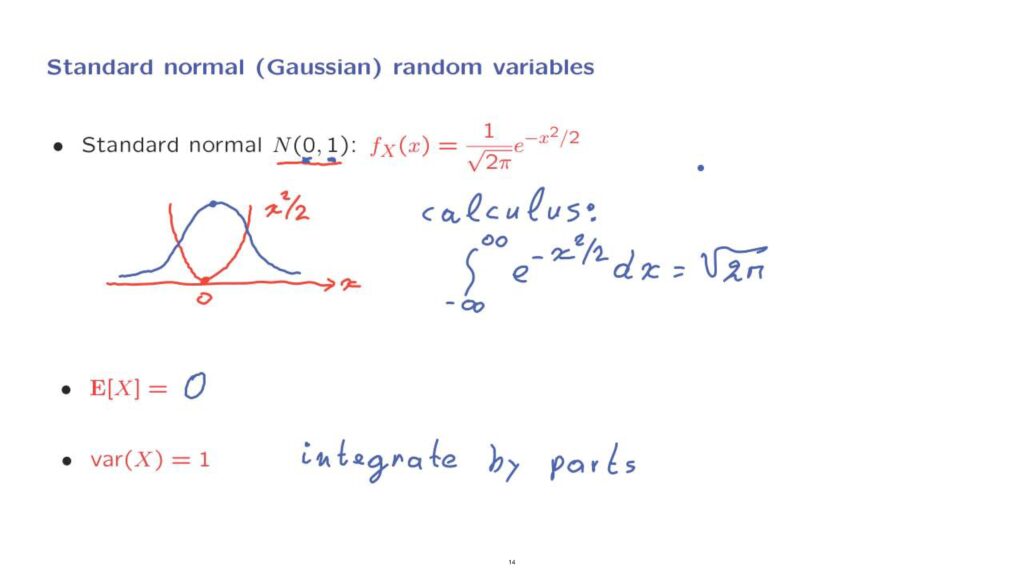
We define normal random variables by specifying their PDFs, and we start with the simplest case of the so-called standard normal.
The standard normal is indicated with this shorthand notation, and we will see shortly why this notation is being used.
It is defined in terms of a PDF.
This PDF is defined for all values of x.
x can be any real number.
So this random variable can take values anywhere on the real line.
And the formula for the PDF is this one.
Let us try to understand this formula.
So we have the exponential of negative x squared over 2.
Now, if we are to plot the x squared over 2 function, it has a shape of this form, and it is centered at zero.
But then we take the negative exponential of this function.
Now, when you take the negative exponential, whenever this thing is big, the negative exponential is going to be small.
So the negative exponential would be equal to 1 when x is equal to 0.
But then as x increases, because x squared also increases, the negative exponential will fall off.
And so we obtain a shape of this kind, and symmetrically on the other side as well.
And finally, there is this constant.
Where [is] this constant coming from? Well there’s a nice and not completely straightforward calculus exercise that tells us that the integral from minus infinity to plus infinity of e to the negative x squared over 2, dx, is equal to the square root of 2 pi.
Now, we need a PDF to integrates to 1.
And so for this to happen, this is the constant that we need to put in front of this expression so that the integral becomes 1, and that explains the presence of this particular constant.
What is the mean of this random variable? Well, x squared is symmetric around 0, and for this reason, the PDF itself is symmetric around 0.
And therefore, by symmetry, the mean has to be equal to 0.
And that explains this entry here.
How about the variance? Well, to calculate the variance, you need to solve a calculus problem again.
You need to integrate by parts.
And after you carry out the calculation, then you find that the variance is equal to 1, and that explains this entry here in the notation that we have been using.
Let us now define general normal random variables.
General normal random variables are once more specified in terms of the corresponding PDF, but this PDF is a little more complicated, and it involves two parameters– mu and sigma squared, where sigma is a given positive parameter.
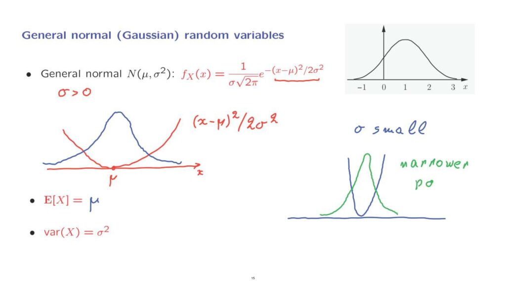
Once more, it will have a bell shape, but this bell is no longer symmetric around 0, and there is some control over the width of it.
Let us understand the form of this PDF by focusing first on the exponent, exactly as we did for the standard normal case.
The exponent is a quadratic, and that quadratic is centered at x equal to mu.
So it vanishes when x is equal to mu, and becomes positive elsewhere.
Then we take the negative exponential of this quadratic, and we obtain a function which is largest at x equal to mu, and falls off as we go further away from mu.
What is the mean of this random variable? Since this term is symmetric around mu, the PDF is also symmetric around mu, and therefore, the mean is also equal to mu.
How about the variance? It turns out– and this is a calculus exercise that we will omit– that the variance of this PDF is equal to sigma squared.
And this explains this notation here.
We’re dealing with a normal that has a mean of mu and a variance of sigma squared.
To get a little bit of understanding of the role of sigma in the form of this PDF, let us consider the case where sigma is small, and see how the picture is going to change.
When sigma is small, and we plot the quadratic, sigma being small means that this quadratic becomes larger, so it rises faster, so we get a narrower quadratic.
And in that case, the negative exponential is going to fall off much faster.
So when sigma is small, the PDF that we get is a narrower PDF, and that reflects itself into the property that the variance will also be smaller.
An important property of normal random variables is that they behave very nicely when you form linear functions of them.
And this is one of the reasons why they’re analytically tractable and analytically very convenient.
Here is what I mean.
Let us start with a normal random variable with a given mean and variance, and let us form a linear function of that random variable.
What is the mean of Y? Well, we know what it is.
We have a linear function of a random variable.
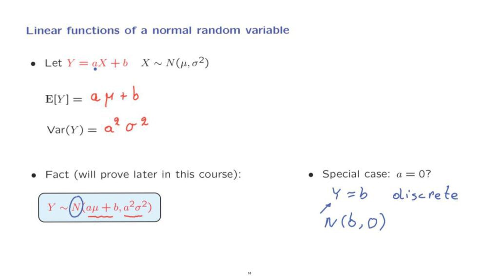
The mean is going to be a times the expected value of X, which is mu plus b.
What is the variance of Y? We know what is the variance of a linear function of a random variable.
It is a squared times the variance of X, which in our case is sigma squared.
So there’s nothing new so far, but there is an additional important fact.
The random variable Y, of course, has the mean and variance that we know it should have, but there is an additional fact– namely, that Y is a normal random variable.
So normality is preserved when we form linear functions.
There’s one special case that’s we need to pay some attention to.
Suppose that a is equal to 0.
In this case, the random variable Y is just equal to b.
It’s a constant random variable.
It does not have a PDF.
It is a degenerate discrete random variable.
So could this fact be correct that Y is also normal? Well, we’ll adopt this as [a] convention.
When we have a discrete random variable, which is constant, it takes a constant value.
We can think of this as a special degenerate case of the normal with mean equal to b and with variance equal to 0.
Even though it is discrete, not continuous, we will still think of it as a degenerate type of a normal random variable, and by adopting this convention, then it will always be true that a linear function of a normal random variable is normal, even if a is equal to 0.
Now that we have the definition and some properties of normal random variables, the next question is whether we can calculate probabilities associated with normal random variables.
This will be the subject of the next segment.