We now introduce a new of random variable, the exponential random variable.
It has a probability density function that is determined by a single parameter lambda, which is a positive number.
And the form of the PDF is as shown here.
Note that the PDF is equal to 0 when x is negative, which means that negative values of X will not occur.
They have zero probability.
And so our random variable is a non-negative random variable.
The shape of the PDF is as shown in this diagram.
It’s 0 for negative values, and then for positive values, it starts off, it starts off at a value equal to lambda.
This is because if you plug in x equal to 0 in this expression, you get lambda times e to the 0, which leaves you just with lambda.
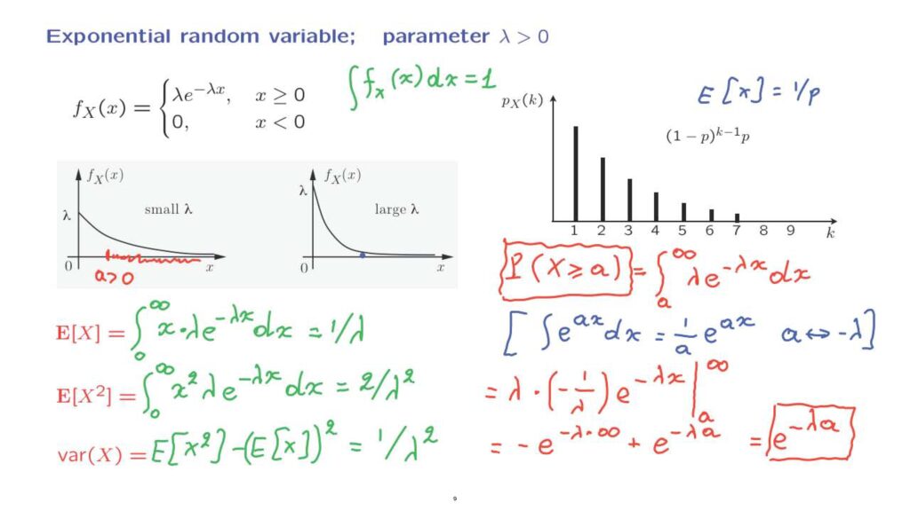
So it starts off with lambda, and then it decays at the rate of lambda.
Notice that when lambda is small, the initial value of the PDF is small.
But then the decay rate is also small, so that the PDF extends over a large range of x’s.
On the other hand, when lambda is large, then the PDF starts large, so there’s a fair amount of probability in the vicinity of 0.
But then it decays pretty fast, so there’s much less probability for larger values of x.
Another observation to make is that the shape of this exponential PDF is quite similar to the shape of the geometric PDF that we have seen before, the only difference being that here we have a discrete distribution, but here we have a continuous analog of that distribution.
Let’s now carry out a calculation.
Let us fix some positive number a, and let us calculate the probability that our random variable takes a value larger than or equal to a.
So what we’re trying to do is to calculate the probability that the random variable falls inside this interval from a to infinity.
Whenever we have a PDF, we can calculate the probability of falling inside an interval by integrating over that interval the value of the PDF.
Therefore, we have to calculate this particular integral.
And at this point, we can recall a fact from calculus, namely that the integral of the function e to the ax is 1 over a times e to the ax.
We can use this fact by making the correspondence between a and minus lambda.
And using this correspondence, we can now continue the calculation of our integral.
We have a factor of lambda.
And then a factor of 1 over a, where a stands for minus lambda.
So we get the minus 1 over lambda.
And then the same exponential function, e to the minus lambda x.
And because the range of integration is from a to infinity, we need to evaluate the integral at a and infinity and take the difference.
Now, this lambda cancels that lambda.
We’re left with a minus sign.
And from the upper limit, we get e to the minus lambda times infinity.
And then from the second term, we have a minus sign that cancels with that minus sign and gives us a plus term, plus e to the minus lambda a.
Now, e to the minus infinity is 0.
And so we’re left just with the last term.
And the answer is e to the minus lambda a.
So this gives us the tail probability for an exponential random variable.
It tells us that the probability of falling higher than a certain number falls off exponentially with that certain number.
An interesting additional observation– if we let a equal to 0 in this calculation, we obtain the integral of the PDF over the entire range of x’s.
And in that case, this probability becomes e to the minus lambda 0, which is equal to 1.
So we have indeed verified that the integral of this PDF is equal to 1, as it should be.
Now, let’s move to the calculation of the expected value of this random variable.
We can use the definition.
Since the PDF is non-zero only for positive values of x, we only need to integrate from 0 to infinity.
We integrate x times the PDF.
And this is an integral that you may have encountered at some point before.
It is evaluated by using integration by parts.
And the final answer turns out to be 1 over lambda.
Regarding the calculation of the expected value of the square of the random variable, we need to write down a similar integral, except that now we will have here x squared.
This is just another integration by parts, only a little more tedious.
And the answer turns out to be 2 over lambda squared.
Finally, to calculate the variance, we use the handy formula that we have.
And the expected value of X squared is this term.
The expected value of X is this term.
When we square it, it becomes similar to this term, but we have here a 2.
There we have a 1.
And so we’re left with just 1 over lambda squared.
And this is the variance of the exponential random variable.
Notice that when lambda is small, the PDF, as we discussed before, falls off very slowly, which means that large x’s are also quite possible.
And so the average of this random variable will be on the higher side.
The PDF extends over a large range, and that translates into having a large mean.
And because when that happens, the PDF actually spreads, the variance also increases.
And this is reflected in this formula for the variance.
The exponential random variable is, in many ways, similar to the geometric.
For example, the expression for the mean, which is 1 over lambda, can be contrasted with the expression for the mean of the geometric, which is 1 over p.
And the relationship between these two distributions, the discrete and the continuous analog, is a theme that we will revisit several times.
At this point, let me just say that the exponential random variable is used to model many important and real world phenomena.
Generally, it models the time that we have to wait until something happens.
In the discrete case, the geometric random variable models the time until we see a success for the first time.
In the continuous case, an exponential can be used to model the time until a customer arrives, the time until a light bulb burns out, the time until a machine breaks down, the time until you receive an email, or maybe the time until a meteorite falls on your house.