As an example of a mean-variance calculation, we will now consider the continuous uniform random variable which we have introduced a little earlier.
This is the continuous analog of the discrete uniform, for which we have already seen formulas for the corresponding mean and variance.
So let us now calculate the mean or expected value for the continuous case.
The mean is defined as an integral that ranges over the entire real line.
On the other hand, we recognize that the density is equal to 0 outside the interval from a to b, and therefore, there is going to be no contribution to the integral from those x’s outside that interval.
This means that we can integrate just over the interval from a to b.
And inside that interval, the value of the density is 1 over b minus a.
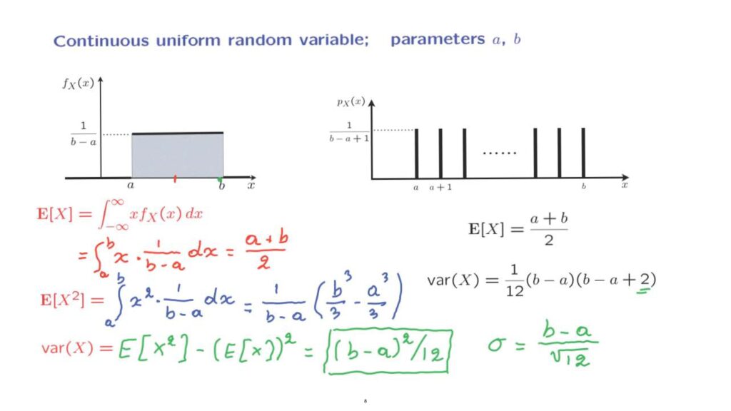
We can carry out this integration and find an answer equal to a plus b over 2, which, interestingly, also happens to be the same as in the discrete case.
In fact, we could find this answer without having to run this integration.
We could just recognize that this PDF is symmetric around the midpoint of the interval, and the midpoint is a plus b over 2.
We now continue with what is involved in the calculation of the expected value of the square of the random variable.
Using the expected value rule, this is the integral of x squared times the density, but because of the same argument as before, we only need to integrate from a to b.
We can evaluate this integral, and the answer turns out to be 1 over (b minus a) times (b cube over 3 minus a cube over 3).
The reason why these cubic terms appear is that the integral of the x square function is x cube divided by 3.
Now that we have this quantity available, we’re ready to calculate the variance using this alternative formula, which, as we have often discussed, usually provides us a quicker way to carry out the calculation.
We take this term, insert it here.
We take the square of this term, insert it here.
Carry out some algebra, and eventually we find an answer which is equal to b minus a squared over 12.
And this is the formula for the variance of a uniform random variable.
We can take the square root of this expression to find the standard deviation, and the standard deviation is going to be b minus a divided by the square root of 12.
A few observations.
First, the formula looks quite similar to the formula for the variance that we had in the discrete case, except that in the discrete case, we have this extra additive factor of 2.
More interestingly, and perhaps more important, is that the standard deviation is proportional to the width of this uniform.
The wider it is, the larger the standard deviation will be.
And this conforms to our intuition that the standard deviation captures the width of a particular distribution.
And the variance, of course, becomes larger when the width is larger.
And as far as the variance is concerned, it increases with the square of the length of the interval over which we have our distribution.