We now start with our agenda of developing continuous counterparts of everything we have done for discrete random variables.
Let us look at the concept of expectation.
In the discrete case, we have defined expectation as a weighted average of the values X of the random variable, weighted according to their corresponding probabilities.
In the continuous case, we define expectation in a similar way– as a weighted average over the possible values of X, weighted according to the corresponding value of the density.
Points where the density is higher– for example, here– will receive a higher weight in this calculation.
But of course, since we are averaging over a continuous set, the summation will have to be replaced by an integral.
This will be a recurrent theme in this unit.
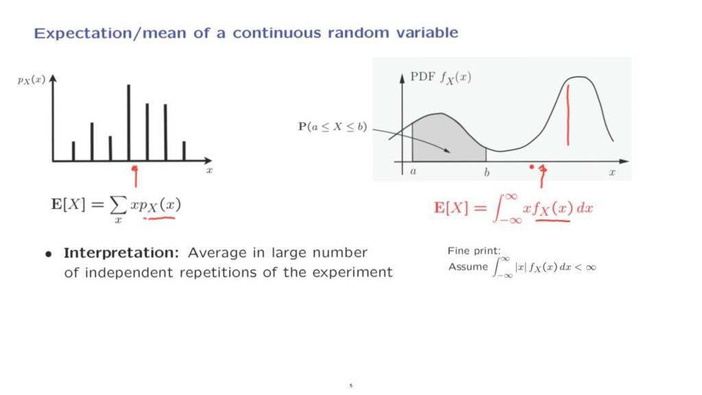
Definitions or formulas for the continuous case look exactly like the discrete ones, except that PMFs are replaced by densities, as here.
The PMF is replaced by a density.
And summations are replaced by integrals.
The intuition is usually the same in both the discrete and the continuous case.
However, the intuition is usually much clearer, much easier to visualize in the discrete case.
So the best strategy is to make sure to understand fully the intuition for the discrete case and just rely on it.
At this point, let me add some fine print– a mathematical side point.
This integral or the expectation will not be always well defined.
For this integral to make sense, we will need to make the assumption that the integral of the absolute value of little x, weighted according to the density, gives us a finite result.
Unless we explicitly say something different, we will always assume that we’re dealing with random variables that satisfy this condition.
And so the expectation is well defined mathematically.
Coming back to the big picture, regarding expectations, the intuition remains the same as in the discrete case– that the expectation represents the average of the values we expect to see in a very large number of independent repetitions of the experiment.
In fact, there are also theorems to this effect, but these will have to wait until later in this class when we study limit theorems.
Another intuitive interpretation that is true for both the discrete and the continuous case is that the expectation corresponds to the center of gravity of the probability distribution.
So in this diagram, it might be somewhere around here.
And similarly, for the continuous diagram, the center of gravity might be somewhere around here.
And if it happens that the distribution, the PMF or the PDF, happens to be symmetric around a certain point, then that point will be equal to the expectation.
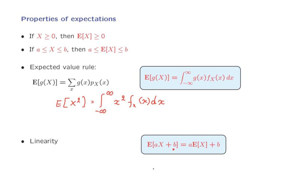
Expectations of continuous random variables have all the properties you might expect.
For example, non-negative random variables have non-negative expectations.
Random variables that lie inside an interval have average values or expectations that also lie inside the same interval.
The derivation is exactly the same as for the discrete case.
There is also an expected value rule.
In the discrete case, it took on this form.
In the continuous case, we obtain an analogous form in which the summation is replaced by [an] integral.
And instead of weighing according to the PMF, we now weigh according to the density function.
The derivation of the expected value rule for the continuous case is a little more complicated than the one that we gave for the discrete case.
But it’s sufficient for us to know that it is true and that it has an intuitive meaning that runs along the same lines as the intuitive meaning that we had for the discrete case.
As an instance of how we might apply the expected value rule, if you wish to calculate the expected value of the square of a continuous random variable, you would proceed as follows.
You would integrate over the entire real line the value of the function, which is X squared in our case, weighted according to the density.
Finally, a most important property of expectations, is linearity.
Linearity is still true for continuous random variables as well.
And the way it is derived is exactly the same as in the discrete case.
Namely, we apply the expected value rule to this function of the random variable X and separate out the various terms.
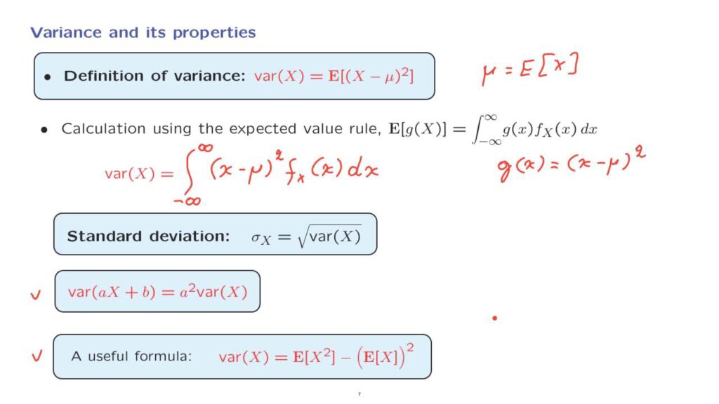
The story regarding variances is exactly the same as in the discrete case.
We define variances using the same definition.
And of course, here, mu stands for the expected value of the random variable X.
To calculate the variance, we can use the expected value rule, which takes this form in the continuous case.
And we apply the expected value rule for the case where we’re dealing with the expected value of this particular function, so that in this instance, the functions g of x is x minus mu squared.
So by applying the expected value rule, we obtain the integral from minus infinity to infinity, the functions g of x, weighted according to the density, and then we carry out the integration.
We also define the standard deviation– same way as in the discrete case.
We have a property about a variance of linear functions, of a random variable, namely, that if we add a constant to a random variable, this has no effect on the variance.
But if we multiply a random variable by a constant, the variance gets multiplied by the square of that constant.
Finally, when calculating the variance, it is often convenient to use this alternative formula in which the variance is calculated by finding the expected value of the square of the random variable and also using the expected value of the random variable, but squared and subtracted from the first term.
This relation and this relation are both derived exactly the same way as in the discrete case.
And there’s no reason to repeat those derivations.