An important reason why conditional probabilities are very useful is that they allow us to divide and conquer.
They allow us to split complicated probability modes into simpler submodels that we can then analyze one at a time.
Let me remind you of the Total Probability Theorem that has his particular flavor.
Total Probability Theorem We divide our sample space into three disjoint events– A1, A2, and A3.
And these events form a partition of the sample space, that is, they exhaust all possibilities.
They correspond to three alternative scenarios, one of which is going to occur.
And then we may be interested in a certain event B.
That event B may occur under either scenario.
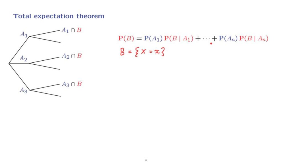
And the Total Probability Theorem tells us that we can calculate the probability of event B by considering the probability that it occurs under any given scenario and weigh those probabilities according to the probabilities of the different scenarios.
Now, let us bring random variables into the picture.
Let us fix a particular value– little x– and let the event B be the event that the random variable takes on this particular value.
Let us now translate the Total Probability Theorem to this situation.
Total Expectation Theorem First, the picture will look slightly different.
Our event B has been replaced by the particular event that we’re now considering.
Now, what is this probability? The probability that event B occurs, having fixed the particular choice of little x, is the value of PMF at that particular x.
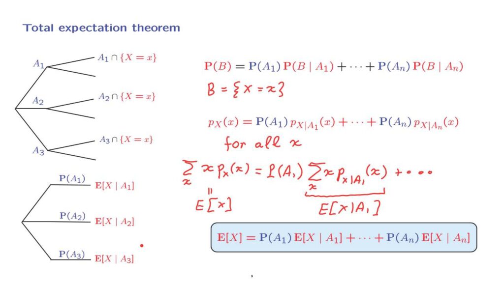
How about this probability here? This is the probability that the random variable, capital X, takes on the value little x– that’s what a PMF is– but in the conditional universe.
So we’re dealing with a conditional PMF.
And so on with the other terms.
So this equation here is just the usual Total Probability Theorem but translated into PMF notation.
Now this version of the Total Probability Theorem, of course, is true for all values of little x.
This means that we can now multiply both sides of this equation by x and them sum over all possibles choices of x.
We recognize that here we have the expected value of the random variable X.
Now, we do the same thing to the right hand side.
We multiply by x.
And then we sum over all possible values of x.
This is going to be the first term.
And then we will have similar terms.
Now, what do we have here? This expression is just the conditional expectation of the random variable X under the scenario that event A1 has occurred.
So what we have established is this particular formula, which is called the Total Expectation Theorem.
It tells us that the expected value of a random variable can be calculated by considering different scenarios.
Finding the expected value under each of the possible scenarios and weigh them.
Weigh the scenarios according to their respective probabilities.
The picture is like this.
Under each scenario, the random variable X has a certain conditional expectation.
We take all these into account.
We weigh them according to their corresponding probabilities.
And we add them up to find the expected value of X.
So we can divide and conquer.
We can replace a possibly complicated calculation of an expected value by hopefully simpler calculations under each one of possible scenarios.
Let me illustrate the idea by a simple example.
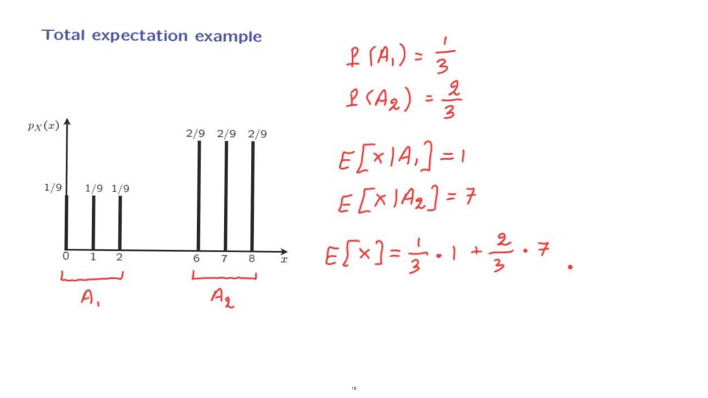
Example Let us consider this PMF, and let us try to calculate the expected value of the associated random variable.
One way to divide and conquer is to define an event, A1, which is that our random variable takes values in this set, and another event, A2, which is that the random variable takes values in that set.
Let us now apply the Total Expectations Theorem.
Let us calculate all the terms that are required.
First, we find the probabilities of the different scenarios.
The probability of event A1 is 1/9 plus 1/9 plus 1/9 which is 1/3.
And the probability of event A2 is 2/9 plus 2/9 plus 2/9 which adds up to 2/3.
How about conditional expectations? In a universe where event A1 one has occurred, only these three values are possible.
They had equal probabilities, so in the conditional model, they will also have equal probabilities.
So we will have a uniform distribution over the set {0, 1, 2}.
By symmetry, the expected value is going to be in the middle.
So this expected value is equal to 1.
And by a similar argument, the expected value of X under the second scenario is going to be the midpoint of this range, which is equal to 7.
And now we can apply the Total Probability Theorem and write that the expected value of X is equal to the probability of the first scenario times the expected value under the first scenario plus the probability of the second scenario times the expected value under the second scenario.
In this case, by breaking down the problem in these two subcases, the calculations that were required were somewhat simpler than if you were to proceed directly.
Of course, this is a rather simple example.
But as we go on with this course, we will apply the Total Probability Theorem in much more interesting and complicated situations.