Discrete Uniform.
In this segment and the next two, we will introduce a few useful random variables that show up in many applications– discrete uniform random variables, binomial random variables, and geometric random variables So let’s start with a discrete uniform.
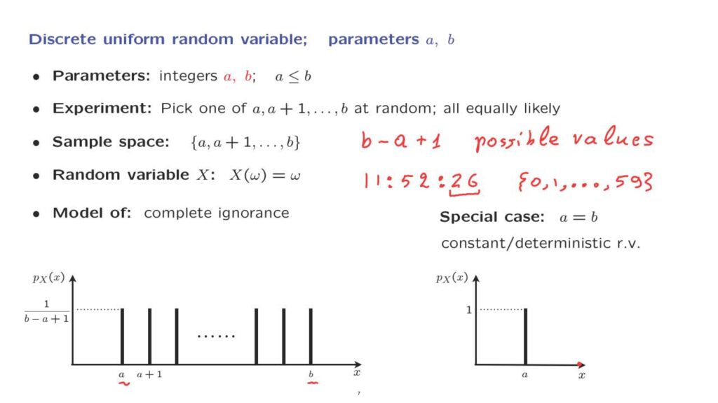
A discrete uniform random variable is one that has a PMF of this form.
It takes values in a certain range, and each one of the values in that range has the same probability.
To be more precise, a discrete uniform is completely determined by two parameters that are two integers, a and b, which are the beginning and the end of the range of that random variable.
Sample Space.
We’re thinking of an experiment where we’re going to pick an integer at random among the values that are between a and b with the end points a and b included.
And all of these values are equally likely.
To be more formal, our sample space is the set of integers from a until b.
And the number of points that we have in our sample space is b minus a plus 1 possible values.
Random Variable What is the random variable that we’re talking about? If this is our sample space, the outcome of the experiment is already a number.
And the numerical value of the random variable is just the number that we happen to pick in that range.
So in this context, there isn’t really a distinction between the outcome of the experiment and the numerical value of the random variable.
They are one in the same.
Now since each one of the values is equally likely, and since we have so many possible values, this means that the probability of any particular value is going to be 1 over b minus a plus 1.
This is the choice for the probability that would make all the probabilities in the PMF sum to one.
What does this random variable model in the real world? It models a case where we have a range of possible values, and we have complete ignorance, no reason to believe that one value is more likely than the other.
As an example, suppose that you look at your digital clock, and you look at the time.
And the time that it tells you is 11:52 and 26 seconds.
And suppose that you just look at the seconds.
The seconds reading is something that takes values in the set from 0 to 59.
So there are 60 possible values.
And if you just choose to look at your clock at a completely random time, there’s no reason to expect that one reading would be more likely than the other.
All readings should be equally likely, and each one of them should have a probability of 1 over 60.
One final comment– let us look at the special case where the beginning and the endpoint of the range of possible values is the same, which means that our random variable can only take one value, namely that particular number a.
In that case, the random variable that we’re dealing with is really a constant.
It doesn’t have any randomness.
It is a deterministic random variable that takes a particular value of a with probability equal to 1.
It is not random in the common sense of the world, but mathematically we can still consider it a random variable that just happens to be the same no matter what the outcome of the experiment is.