A random variable can take different numerical values depending on the outcome of the experiment.
Some outcomes are more likely than others, and similarly some of the possible numerical values of a random variable will be more likely than others.
We restrict ourselves to discrete random variables, and we will describe these relative likelihoods in terms of the so-called probability mass function, or PMF for short, which gives the probability of the different possible numerical values.
The PMF is also sometimes called the probability law or the probability distribution of a discrete random variable.
Let me illustrate the idea in terms of a simple example.
We have a probabilistic experiment with four possible outcomes.
We also have a probability law on the sample space.
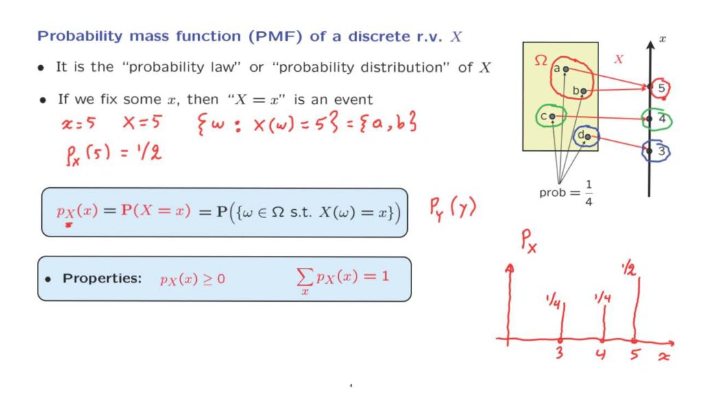
And to keep things simple, we assume that all four outcomes in our sample space are equally likely.
We then introduce a random variable that associates a number with each possible outcome as shown in this diagram.
The random variable, X, can take one of three possible values– namely 3, 4, or 5.
Let us focus on one of those numbers– let’s say the number 5.
So let us focus on x being equal to 5.
We can think of the event that X is equal to 5.
Which event is this? This is the event that the outcome of the experiment led to the random variable taking a value of 5.
So it is this particular event which consists of two elements, namely a and b.
More formally, the event that we’re talking about is the set of all outcomes for which the value, the numerical value of our random variable, which is a function of the outcome, that numerical value happens to be equal to 5.
And in this example it is a set consisting of two elements.
It’s a subset of the sample space.
So it is an event.
And it has a probability.
And that probability we will be denoting with this notation.
And in our case this probability is equal to 1/2.
Because we have two outcomes, each one has probability 1/4.
The probability of this event is equal to 1/2.
More generally, we will be using this notation to denote the probability of the event that the random variable, X , takes on a particular value, x.
This is just a piece of notation, not a new concept.
We’re dealing with a probability, and we indicate it using this particular notation.
More formally, the probability that we’re dealing with is the probability, the total probability, of all outcomes for which the numerical value of our random variable is this particular number, x.
A few things to notice.
We use a subscript, X, to indicate which random variable we’re talking about.
This will be useful if we have several random variables involved.
For example, if we have another random variable on the same sample space, Y, then it would have its own probability mass function which would be denoted with this particular notation here.
The argument of the PMF, which is x, ranges over the possible values of the random variable, X.
So in this sense, here we’re really dealing with a function.
A function that we could denote just by p with a subscript x.
This is a function as opposed to the specific values of this function.
And we can produce plots of this function.
In this particular example that we’re dealing with, the interesting values of x are 3, 4, and 5.
And the associated probabilities are the value of 5 is obtained with probability 1/2, the value of 4– this is the event that the outcome is c, which has probability 1/4.
And the value of 3 is also obtained with probability 1/4 because the value of 3 is obtained when the outcome is d, and that outcome has probability 1/4.
So the probability mass function is a function of an argument x.
And for any x, it specifies the probability that the random variable takes on this particular value.
A few more things to notice.
The probability mass function is always non-negative, since we’re talking about probabilities and probabilities are always non-negative.
In addition, since the total probability of all outcomes is equal to 1, the probabilities of the different possible values of the random variable should also add to 1.
So when you add over all possible values of x, the sum of the associated probabilities should be equal to 1.
In terms of our picture, the event that x is equal to 3, which is this subset of the sample space, the event that x is equal to 4, which is this subset of the sample space, and the event that x is equal to 5, which is this subset of the sample space.
These three events– the red, green, and blue– they are disjoint, and together they cover the entire sample space.
So their probabilities should add to 1.
And the probabilities of these events are the probabilities of the different values of the random variable, X.
So the probabilities of these different values should also add to 1.
Let us now go through a simple example to illustrate the general method for calculating the PMF of a discrete random variable.
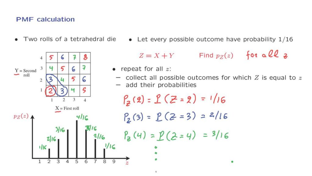
We will revisit our familiar example involving two rolls of the tetrahedral die.
And let X be the result of the first roll, Y be the result of the second roll.
And notice that we’re using uppercase letters.
And this is because X and Y are random variables.
In order to do any probability calculations, we also need the probability law.
So to keep things simple, let us assume that every possible outcome, there’s 16 of them, has the same probability which is therefore 1 over 16 for each one of the outcomes.
We will concentrate on a particular random variable defined to be the sum of the random variables, X and Y.
So if X and Y both happen to be 1, then Z will take the value of 2.
If X is 2 and Y is 1 our random variable will take the value of 3.
And similarly if we have this outcome, in those outcomes here, the random variable takes the value of 4.
And we can continue this way by marking, for each particular outcome, the corresponding value of the random variable of interest.
What we want to do now is to calculate the PMF of this random variable.
What does it mean to calculate the PMF? We need to find this value for all choices of z, that is for all possible values in the range of our random variable.
The way we’re going to do it is to consider each possible value of z, one at a time, and for any particular value find out what are the outcomes– the elements of the sample space– for which our random variable takes on the specific value, and add the probabilities of those outcomes.
So to illustrate this process, let us calculate the value of the PMF for z equal to 2.
This is by definition the probability that our random variable takes the value of 2.
And this is an event that can only happen here.
It corresponds to only one element of the sample space, which has probability 1 over 16.
We can continue the same way for other values of z.
So for example, the value of PMF at z equal to 3, this is the probability that our random variable takes the value of 3.
This is an event that can happen in two ways– it corresponds to two outcomes– and so it has probability 2 over 16.
Continuing similarly, the probability that our random variable takes the value of 4 is equal to 3 over 16.
And we can continue this way and calculate the remaining entries of our PMF.
After you are done, you end up with a table– or rather a graph– a plot that has this form.
And these are the values of the different probabilities that we have computed.
And you can continue with the other values.
It’s a reasonable guess that this was going to be 4 over 16, this is going to be 3 over 16, 2 over 16, and 1 over 16.
So we have completely determined the PMF of our random variable.
We have given the form of the answers.
And it’s always convenient to also provide a plot with the answers that we have.