We now come to the third and final kind of calculation out of the calculations that we carried out in our earlier example.
The setting is exactly the same as in our discussion of the total probability theorem.
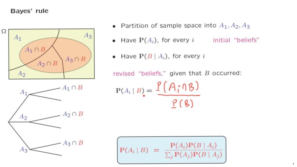
We have a sample space which is partitioned into a number of disjoint subsets or events which we think of as scenarios.
We’re given the probability of each scenario.
And we think of these probabilities as being some kind of initial beliefs.
They capture how likely we believe each scenario to be.
Now, under each scenario, we also have the probability that an event of interest, event B, will occur.
Then the probabilistic experiment is carried out.
And perhaps we observe that event B did indeed occur.
Once that happens, maybe this should cause us to revise our beliefs about the likelihood of the different scenarios.
Having observed that B occurred, perhaps certain scenarios are more likely than others.
How do we revise our beliefs? By calculating conditional probabilities.
And how do we calculate conditional probabilities? We start from the definition of conditional probabilities.
The probability of one event given another is the probability that both events occur divided by the probability of the conditioning event.
How do we continue? We simply realize that the numerator is what we can calculate using the multiplication rule.
And the denominator is exactly what we calculate using the total probability theorem.
So we have everything we need to calculate those revised beliefs, or conditional probabilities.
And this all there is in the Bayes rule.
It is actually a very simple calculation.
It’s a very simple calculation.
However, it is a quite important one.
Its history goes way back.
In the middle of the 18th century, a Presbyterian minister, Thomas Bayes, worked it out.
It was published a few years after his death.
And it was quickly reorganized for its significance.
It’s a systematic way for incorporating new evidence.
It’s a systematic way for learning from experience.
And it forms the foundation of a major branch of mathematics, so-called Bayesian inference, which we will study in some detail later in this course.
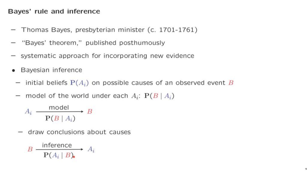
The general idea is that we start with a probabilistic model, which involves a number of possible scenarios.
And we have some initial beliefs on the likelihood of each possible scenario.
There’s also some particular event that may occur under each scenario.
And we know how likely it is to occur under each scenario.
This is our model of the situation.
Under each particular situation, the model tells us how likely event B is to occur.
If we actually observe that B occurred, then we use that information to draw conclusions about the possible causes of B, or conclusions about the more likely or less likely scenarios that may have caused this events to occur.
That’s what inference is.
Having observed b, we make inferences as to how likely a particular scenario, Ai, is going to be.
And that likelihood is captured by this conditional probabilities of Ai, given the event B.
So that’s what the Bayes rule is doing.
Starting from conditional probabilities going in one direction, it allows us to calculate conditional probabilities going in the opposite direction.
It allows us to revise the probabilities of the different scenarios, taking into account the new information.
And that’s exactly what inference is all about, as we’re going to see later in this class.