We have seen so far an example of a probability law on a discrete and finite sample space as well as an example with an infinite and continuous sample space.
Let us now look at an example involving a discrete but infinite sample space. We carry out an experiment whose outcome is an arbitrary positive integer.
As an example of such an experiment, suppose that we keep tossing a coin and the outcome is the number of tosses until we observe heads for the first time.
The first heads might appear in the first toss or the second or the third, and so on. So in this example, any positive integer is possible. And so our sample space is infinite. Let us not specify a probability law.
A probability law should determine the probability of every event, of every subset of the sample space. That is, the probability of every set of positive integers. But instead I will just tell you the probability of events that contain a single element.
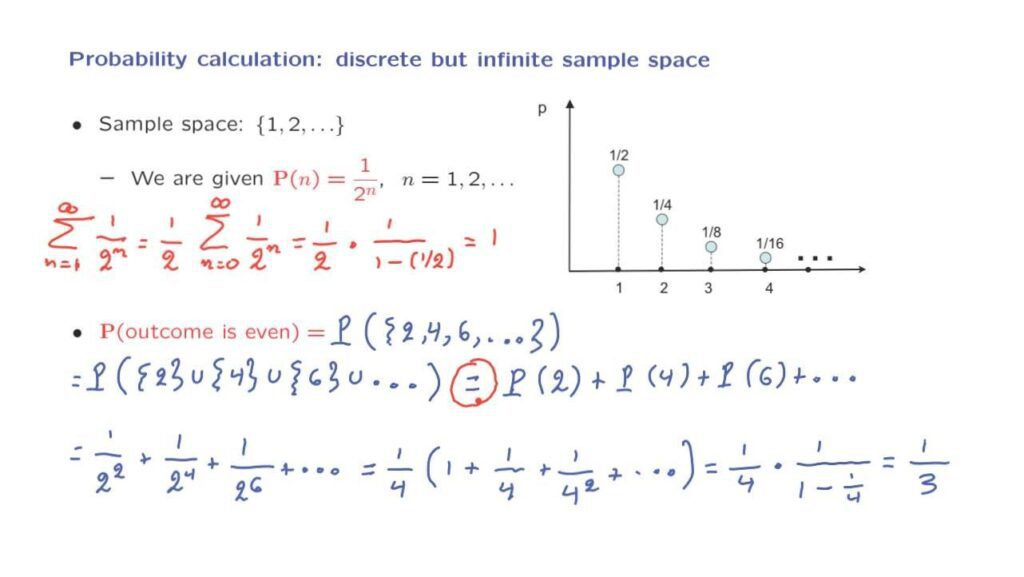
I’m going to tell you that there is probability 1 over 2 to the n that the outcome is equal to n. Is this good enough? Is this information enough to determine the probability of any subset?
Before we look into that question, let us first do a quick sanity check to see whether these numbers that we are given look like legitimate probabilities. Do they add to 1?
Let’s do a quick check. So the sum over all the possible values of n of the probabilities that we’re given, which is an infinite sum starting from 1, all the way up to infinity, of 1 over 2 to the n, is equal to the following. First we take out a factor of 1/2 from all of these terms, which reduces the exponent from n to n minus 1.
This is the same as running the sum from n equals 0 to infinity of 1/2 and to the n. And now we have a usual infinite geometric series and we have a formula for this. The geometric series has a value of 1 over 1 minus the number whose power we’re taking, which is 1/2. And after we do the arithmetic, this turns out to be equal to 1.
So indeed, it appears that we have the basic elements of what it would take to have a legitimate probability law. But now let us look into how we might calculate the probability of some general event. For example, the probability that the outcome is even.
We proceed as follows. The probability that the outcome is even, this is the probability of an infinite set that consists of all the even integers. We can write this set as the union of lots of little sets that contain a single element each.
So it’s the set containing the number 2, the set containing the number 4, the set containing the number 6, and so on.
At this point we notice that we’re talking about the probability of a union of sets and these sets are disjoint because they contain different elements.
So we can use an additivity property and say that this is the probability of obtaining a 2, plus the probability of obtaining a 4, plus the probability of obtaining a 6 and so on.
If you’re curious about doing this calculation and actually obtaining a numerical answer, you would proceed as follows. You notice that this is 1 over 2 to the second power plus 1 over 2 to the fourth power plus 1 over 2 to the sixth power and so on. Now you factor out a factor of 1/4 and what you’re left is 1 plus 1 over 2 to the second power, which is 1/4, plus 1 over 2 to the fourth power, which is the same as 1/4 to the second power and so on.
And now we have 1/4 times the infinite sum of a geometric series, which gives us 1 over 1 minus 1/4. And after you do the algebra you obtain a numerical answer, which is equal to 1/3.
But leaving the details of the calculation aside, the more important question I want to address is the following. Is this calculation correct?
We seem to have used an additivity property at this point.
But the additivity properties that we have in our hands at this point only talk about disjoint unions of finitely many subsets.
Our initial axiom talked about a disjoint union of two subsets and then later on we established a similar property for a disjoint union of finitely many subsets. But here we’re talking about the union of infinitely many subsets.
So this step here is not really allowed by what we have in our hands. On the other hand, we would like our theory to allow this kind of calculation. The way out of this dilemma is to introduce an additional axiom that will indeed allow this kind of calculation.
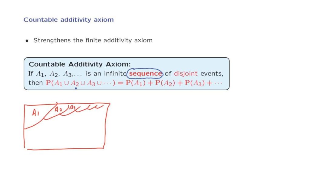
The axiom that we introduce is the following. If we have an infinite sequence of disjoint events, as for example in this picture.
We have our sample space.
We have a first event, A1.
We have a second event, A2.
The third event, A3.
And so we keep continuing and we have an infinite sequence of such events. Then the probability of the union of these events, of these infinitely many events, is the sum of their individual probabilities. The key word here is the word sequence.
Namely, these events, these sets that we’re dealing with, can be arranged so that we can talk about the first event, A1, the second event, A2, the third one, A3, and so on.
To appreciate the issue that arises here and to see why the word sequence is so important, let us consider the following calculation. Our sample space is the unit square. And we consider a model where the probability of a set is its area, as in the examples that we considered earlier.
Let us now look at the probability of the overall sample space. Our sample space is the unit square and the unit square can be thought of as the union of various sets that consist of single points.
So it’s the union of subsets with one element each. And it’s a union taken over all the points in the unit square. Then we think about additivity. We observe that these subsets are disjoint.
If we’re considering different points, then we get disjoint single element sets. And then an additivity property would tells us that the probability of these union is the sum of the probabilities of the different single element subsets. Now, as we discussed before, single element subsets have 0 probability.
So we have a sum of lots of 0s and the sum of 0s should be equal to 0. On the other hand, by the probability axioms, the probability of the entire sample space should be equal to 1.
And so we have established that 1 is equal to 0. This looks like a paradox.
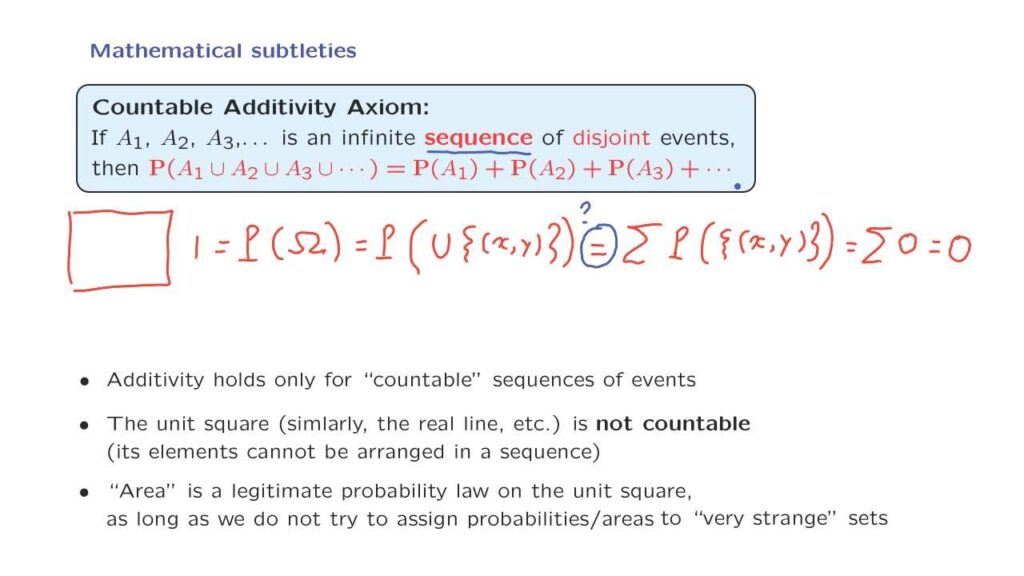
Is it? The catch is that there is nothing in the axioms we have introduced so far or the properties we have established that would justify this step. So this step here is questionable.
You might argue that the unit square is the union of disjoint single element sets, which is the case that we have in additivity axioms. But the additivity axiom only applies when we have a sequence of events. And this is not what we have here. This is not a union of a sequence of single element sets.
In fact, there is no way that the elements of the unit square can be arranged in a sequence. The unit square is said to be an uncountable set. This is a deep and fundamental mathematical fact.
What it essentially says is that there are two kinds of infinite sets. Discrete ones or in formal terminology countable. These are sets whose elements can be arranged in a sequence, like the integers. And also uncountable sets, such as the unit square or the real line, whose elements cannot be arranged in a sequence.
If you’re curious, you can find the proof of this important fact in the supplementary materials that we are providing. After all these discussion, you may now have legitimate suspicions about the models we have been looking at. Is area a legitimate probability law? Does it even satisfy countable additivity?
This question takes us into deep waters and has to do with a deep subfield of mathematics called Measure Theory. Fortunately, it turns out that all is well. Area is a legitimate probability law. It does indeed satisfy the countable additivity axiom as long as we only deal with nice subsets of the unit square. Fortunately, the subsets that arise in whatever we do in this course will be “nice”.
Subsets that are not nice are quite pathological and we will not encounter them. At this stage we are not in a position to say anything more that would be meaningful about these issues because they’re quite complicated and mathematically deep.
We can only say that there are some serious mathematical subtleties. But fortunately, they can all be overcome in a rigorous manner. And for the rest of this class, you can just forget about these subtle issues.