The trajectory estimation problem that we considered gives you a first glimpse into a large field that deals with linear normal models.
In this segment, I will just give you a preview of what happens in that field, although, we will not attempt to prove or justify anything.
What happens in this field is that we’re dealing with models where there are some underlying independent normal random variables.
And then, the random variables of interest, the unknown parameters and the observations, can all be expressed as linear functions of these independent normals.
Since linear functions of independent normals are normal, in particular, this means that the Theta j and the Xi are all normal random variables.
Carrying out inference within this class of models goes under the name of linear regression.
One can proceed using pretty much the same steps as we had in the trajectory estimation problem and write down formulas for the posterior.
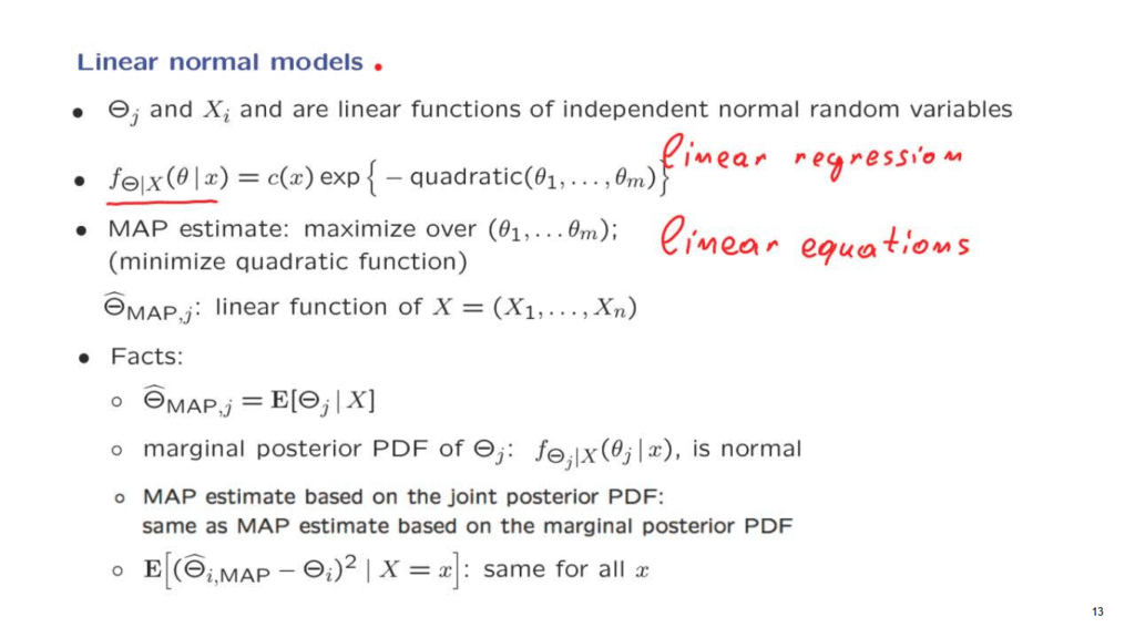
And it turns out that in every case, the posterior of the parameter vector takes a form which is the exponential of and the negative of a quadratic function of the parameters.
And this means, in particular, that in order to find the MAP estimate of the vector Theta, what we need to do is to just minimize this quadratic function with respect to theta.
And minimizing a quadratic function is done by taking derivatives and setting them to zero which leads us to a system of linear equations, exactly as in the trajectory inference problem.
And this means that numerically it is very simple to come up with a MAP estimate.
There’s an interesting fact that comes out of the algebra involved, namely, that the MAP estimate of each one of the parameters turns out to also be a linear function of the observations.
We saw this property in the estimators that we derived for simpler cases in this lecture sequence.
It turns out that this property is still true.
And this is an appealing and desirable property because it means that these estimators can be applied very efficiently in practice without having to do any complicated calculations.
Finally, there’s a number of important facts, some of which we have seen in our examples which are true in very big generality.
One fact is that the maximum a posteriori probability estimate of some parameter turns out to be the same as the conditional expectation of that parameter.
Furthermore, if you look at this joint density of all the Theta parameters and from it you find the marginal density of the Theta parameters always within this conditional universe.
It turns out that this marginal posterior PDF is itself normal.
Since it is normal, its mean– which is this quantity– is going to be equal to its peak.
And therefore, it is equal also to the MAP estimate that would be derived from this marginal PDF.
So what do we have here?
There are two ways of coming up with MAP estimates.
One way is to find the peak of the joint PDF, and then read out the different components of Theta.
Another way of coming up with MAP estimates is to find for each parameter the marginal PDF and look at the peak of this marginal PDF.
It turns out that for this model these two approaches are going to give you the same answer.
Whether you work with the marginal or with the joint, you get the same MAP estimates.
And this is a reassuring property to have.
Finally, as in the examples that we have worked in more detail, it turns out that the mean squared error conditioned on a particular observation is the same no matter what the value of that observation was.
And furthermore, there are fairly simple and easily computable formulas that one can apply in order to find what this mean squared error is.
So to summarize, this class of models that involve linear relations and normal random variables have a rich set of important and elegant properties.
This is one of the reasons why these models are used very much in practice.
And they’re probably the most widely used class of statistical models.