In this segment, we introduce a model with multiple parameters and multiple observations.
It is a model that appears in countless real-world applications.
But instead of giving you a general and abstract model, we will talk about a specific context that has all the elements of the general model, but it has the advantage of being concrete.
And we can also visualize the results.
The model is as follows.
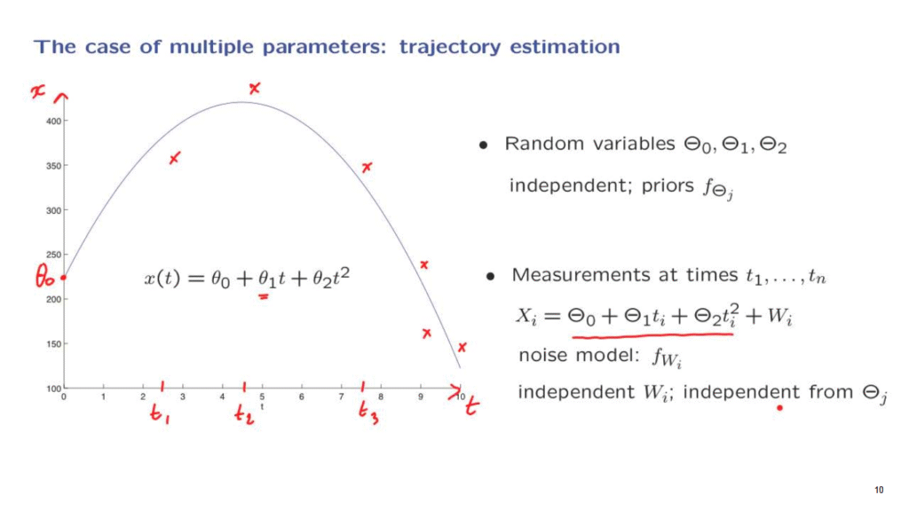
Somebody is holding a ball and throws it upwards.
This ball is going to follow a certain trajectory.
What kind of trajectory is it?
According to Newton’s laws, we know that it’s going to be described by a quadratic function of time.
So here’s a plot of such a quadratic function, where this is the time axis.
And this variable here, x, is the vertical displacement of the ball.
The ball initially is it a certain location, at a certain height– theta 0.
It is thrown upwards.
And it starts moving with some initial velocity, theta 1.
But because of the gravitational force, it will start eventually going down.
So this parameter theta 2, which would actually be negative, reflects the gravitational constant.
Suppose now that you do not know these parameters.
You do not to know exactly where the ball was when it was thrown.
You don’t know the exact velocity.
And perhaps you also live in a strange gravitational environment, and you do not know the gravitational constant.
And you would like to estimate those quantities based on measurements.
If you are to follow the Bayesian Inference methodology, what you need to do is to model those variables as random variables, and think of the actual realized values as realizations of these random variables.
And we also need some prior distributions for these random variable.
We should specify the joint PDF of these three random variables.
A common assumption here is to assume that the random variables involved are independent of each other.
And each one has a certain prior.
Where do these priors come from?
If for example you know where is the person that’s throwing the ball, if you know their location within let’s say a meter or so, you should have a distribution for Theta 0 that describes your state of knowledge and which has a width or standard deviation of maybe a couple of meters.
So the priors are chosen to reflect whatever you know about the possible values of these parameters.
Then what is going to happen is that you’re going to observe the trajectory at certain points in time.
For example, at a certain time t1, you make a measurement.
But your measurement is not exact.
It is noisy, and you record a certain value.
At another time you make another measurement, and you record another value.
At another time, you make another measurement, and you record another value.
And similarly, you get multiple measurements.
On the basis of these measurements, you would like to estimate the parameters.
Let us write down a model for these measurements.
We assume that the measurement is equal to the true position of the ball at the time of the measurement, which is this quantity, plus some noise.
And we introduce a model for these noise random variables.
We assume that we have a probability distribution for them.
And we also assume that they’re independent of each other, and independent from the Thetas.
It is quite often that measuring devices, when they try to measure something multiple times, the corresponding noises will be independent.
So this is often a realistic assumption.
And in addition, the noise in the measuring devices is usually independent from whatever randomness there is that determined the values of the phenomenon that you are trying to measure.
So these are pretty common and realistic assumptions.
Let us take stock of what we have.
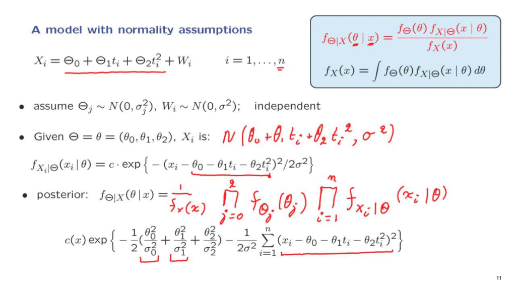
We have observations that are determined according to this relation, where Wi are noise terms.
Now let us make some more concrete assumptions.
We will assume that the random variables, the Thetas, are normal random variables.
And similarly, the W’s are normal.
As we said before, they’re all independent.
And to keep the formula simple, we will assume that the means of those random variables are 0, although the same procedure can be followed if the means are non-0.
We would like to estimate the Theta parameters on the basis of the observations.
We will use as usual, the appropriate form of the Bayes rule, which is this one– the Bayes rule for continuous random variables.
The only thing to notice is that in this notation here, x is an n-dimensional vector, because we have n observations.
And theta in this example is a three-dimensional vector, because we have three unknown parameters.
So wherever you see a theta or an x without a subscript, it should be interpreted as a vector.
Now, in order to calculate this posterior distribution, we need to put our hands on the conditional density of X.
Actually, it’s a joint density, because X is a vector given the value of Theta.
The arguments are pretty much the same as in our previous examples.
And it goes as follows.
Suppose that I tell you the value of the parameters, as here.
Then we look at this equation.
This quantity is now a constant.
And we have a constant plus normal noise.
So Xi is this normal noise whose mean is shifted by this constant.
So Xi is going to be a normal random variable, with a mean of theta 0 plus theta 1ti, plus theta 2ti squared.
And a variance equal to the variance of Wi.
We know what the normal PDF is.
So we can write it down.
It’s the usual exponential of a quadratic.
And in this quadratic, we have Xi minus the mean of the normal random variable that we’re dealing with.
Let us now continue and write down a formula for the posterior.
We first have this denominator term, which does not involve any thetas, and as in previous examples, does not really concern us.
Here we have the joint PDF of the vector of Thetas.
There’s three of them.
Because we assumed that the Thetas are independent, the joint PDF factors as a product of individual PDFs.
And then, we have here the joint PDF of X, conditioned on Theta.
Now with the same argument is in our previous discussion of the case of multiple observations, once I tell you the values of Theta, then the Xi’s are just functions of the noises.
The noises are independent, so the Xi’s are also independent.
So in the conditional universe, where the value of Theta is known, the Xi’s are independent and therefore, the joint PDF of the Xi’s is equal to the product of the marginal PDFs of each one of the Xi’s.
But this marginal PDF in the conditional universe of the Xi’s is something that we have already calculated.
And so we know what each one of these densities is.
We can write them down.
And we obtain an expression of this form.
We have a normalizing constant in the beginning.
We have here a term that comes from the prior for Theta 0, a prior from Theta 1.
Here is a typical term that comes from the density of Xi, which is this term up here.
So here is what we have so far.
How should we now estimate Theta if we wish to derive a point estimate?
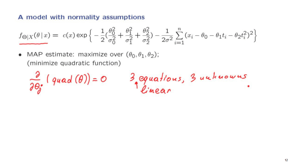
The natural process is to look for the maximum posteriori probability estimate, which will maximize this expression over theta.
Find a set of theta parameters.
It’s a three-dimensional vector for which is this quantity is largest.
Equivalently we can look at the exponent, get rid of the minus signs, and minimize the quadratic function that we obtain here.
How does one minimize a quadratic function?
We take the derivatives with respect to each one of the parameters, and set the derivative to 0.
We will get this way three equations and three unknowns.
And because it’s a quadratic function of theta, these derivatives will be linear functions of theta.
So these equations that we’re dealing with will be linear equations.
So it’s a system of three linear equations which we can solve numerically.
And this is what is usually done in practice.
A this is exactly what it takes to calculate the maximum a posteriori probability estimate in this particular example that we have discussed.
It turns out as we will discuss later, that there are many interesting properties for this estimate, and which are quite general.