We will now continue with the problem of inferring the unknown bias of a certain coin for which we have a certain prior distribution and of which we observe the number of heads in n independent coin tosses.
We have already seen that if we assume a uniform prior, the posterior takes this particular form, which comes from the family of Beta distributions.
What we want to do now is to actually derive point estimates.
That is, instead of just providing the posterior, we would like to select a specific estimate for the unknown bias.
Let us look at the maximum a posteriori probability estimate.
How can we find it?
By definition, the MAP estimate is that value of theta that maximizes the posterior, the value of theta at which the posterior is largest.
Now, instead of maximizing the posterior, it is more convenient in this example to maximize the logarithm of the posterior.
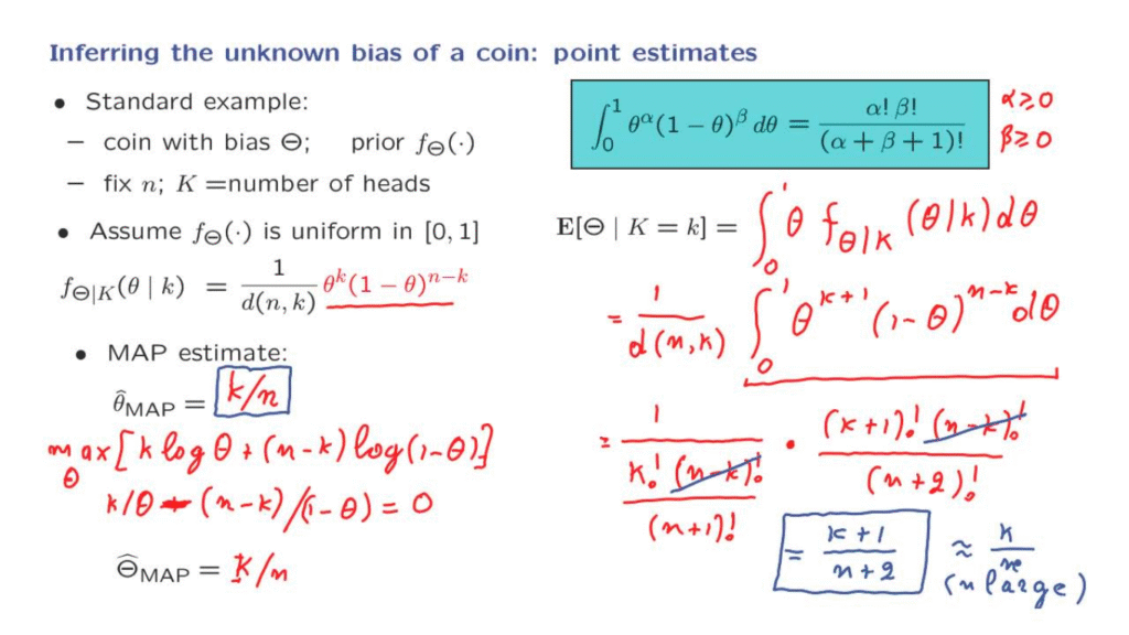
And the logarithm is k times log theta, plus n minus k times the log of 1 minus theta.
To carry out the maximization over theta, we form the derivative with respect to theta and set that derivative to 0.
So the derivative of the first term is k over theta.
And the derivative of the second term is n minus k over this quantity, 1 minus theta.
But because of the minus here when we apply the chain rule, actually, this plus sign here is going to become a minus sign.
And now we set this derivative to 0.
We carry out the algebra, which is rather simple.
And the end result that you will find is that the estimate is equal to k over n.
Notice that this is lowercase k.
We are told the specific value of heads that has been observed.
So little k is a number, and our estimate, accordingly, is a number.
This answer makes perfect sense.
A very reasonable way of estimating the probability of heads of a certain coin is to look at the number of heads obtained and divide by the total number of trials.
So we see that the MAP estimate turns out to be a quite natural one.
How about the corresponding estimator?
Recall the distinction that the estimator is a random variable that tells us what the estimate is going to be as a function of the random variable that is going to be observed.
The estimator is uppercase K divided by little n.
So it is a random variable whose value is determined by the value of the random variable capital K.
If the random variable capital K happens to take on this specific value, little k, then our estimator, this random variable, will be taking this specific value, which is the estimate.
And let us now compare with an alternative way of estimating Theta.
We will consider estimating Theta by forming the conditional expectation of Theta, given the specific number of heads that we have observed.
This is what we call the LMS or least mean squares estimate.
To calculate this conditional expectation, all that we need to do is to form the integral of theta times the density of Theta.
But since it’s a conditional expectation, we need to take the conditional density of Theta.
And the integral ranges from 0 to 1, because this is the range of our random variable, Theta.
Now, what is this?
We have a formula for the posterior density.
So we need to just multiply this expression here by theta, and then integrate.
This term here is a constant.
So it can be pulled outside the integral.
And inside the integral, we are left with this term times theta, which changes the exponent of theta to k plus 1.
Then we have 1 minus theta to the power n minus k, d theta.
At this point, we need to do some calculations.
What is d of n, k?
d of n, k is the normalizing constant of this PDF.
For this to be a PDF and to integrate to 1, d of n, k has to be equal to the integral of this expression from 0 to 1.
So we need to somehow be able to evaluate this integral.
Here, we will be helped by the following very nice formula.
This formula tells us that the integral of for such a function of theta from 0 to 1 is equal to this very nice and simple expression.
Of course, this formula is only valid when these factorials make sense.
So we assume that alpha is non-negative and theta is non-negative.
How is this formula derived?
There’s various algebraic or calculus style derivations.
One possibility is to use integration by parts.
And there are also other tricks for deriving it.
It turns out that there is also a very clever probabilistic proof of this fact.
But in any case, we will not derive it.
We will just take it as a fact that comes to us from calculus.
And now, let us apply this formula.
d of n, k is equal to the integral of this expression, which is of this form, with alpha equal to k and beta equal to n minus k.
So d of n, k takes the form alpha is k, beta is n minus k.
And then in the denominator, we have the sum of the two indices plus 1.
So it’s going to be k plus n minus k.
That gives us n.
And then there’s a plus 1.
And how about this integral?
Well, this integral is also of the form that we have up here.
But now, we have alpha equal to k plus 1, beta is n minus k.
And in the denominator, we have the sum of the indices plus 1.
So when we add these indices, we get n plus 1.
And then we get another factor of 1, which gives us an n plus 2.
This looks formidable.
But actually, there’s a lot of simplifications.
This term here cancels with that term.
k plus 1 factorial divided by k factorial, what is it?
It is just a factor of k plus 1.
And what do we have here?
This term is in the denominator of the denominator.
So it can be moved up to the numerator.
We have n plus 1 factorial divided by n plus 2 factorial.
This is just n plus 2.
And this is the final form of the answer.
This is what the conditional expectation of theta is.
So now, we can compare the two estimates that we have, the MAP estimate and the conditional expectation estimate.
They’re fairly similar, but not exactly the same.
This means that the mean of a Beta distribution is not the same as the point at which the distribution is highest.
On the other hand, if n is a very large number, this expression is going to be approximately equal to k over n when n is large.
And so in the limit of large n, the two estimators will not be very different from each other.