We can finally go ahead and introduce the basic elements of the Bayesian inference framework.
There is an unknown quantity, which we treat as a random variable, and this is what’s special and why we call this the Bayesian inference framework.
This is in contrast to other frameworks in which the unknown quantity theta is just treated as an unknown constant.
But here, we treat it as a random variable, and as such, it has a distribution.
This is the prior distribution.
This is what we believe about Theta before we obtain any data.
And then, we obtain some data, which are some observation.
That observation is a random variable, but when the process gets realized, we observe an actual value, numerical value, of this random variable.
The observation process is modeled, again in terms of a probabilistic model.
We specify the distribution of X, but we actually specify the conditional distribution of X.
We say how X will behave if Theta happens to take on a specific value.
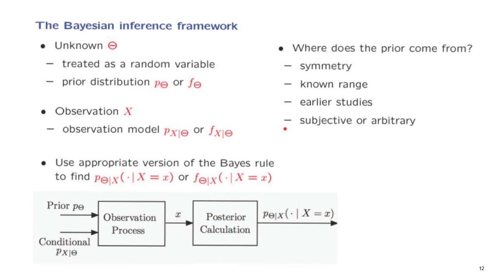
These two pieces, the prior and the model of the observations, are the two components of the model that we will be working with.
Once we have obtained a specific value for the observations, then we can use the Bayes rule to calculate the conditional distribution of Theta, either a conditional PMF if Theta is discrete or a conditional PDF if Theta is continuous.
And this will be a complete solution, in some sense, of the Bayesian inference problem.
There’s one philosophical issue about this framework, which is where does this prior distribution come from?
How do we choose it?
Sometimes we can choose it using a symmetry argument.
If there’s a number of possible choices for Theta and there’s a reason to believe that they’re all equally likely, we have no reason to believe that one is more likely than the other, then the symmetry consideration gives us a uniform prior.
We definitely take into account any information we have about the range of the parameter Theta, so we use that range and we assign 0 prior probability for values of Theta outside the range.
Sometimes, we have some knowledge about Theta from previous studies of a certain problem, that tell us a little bit about what Theta might be, and then when we obtain new observations, we refine those results that were obtained from previous studies by applying the Bayes rule.
And in some cases, finally, the choice could be arbitrary or subjective just reflecting our beliefs about Theta, some plausible judgment about the relative likelihoods of different choices of Theta.
Now, as we just discussed, the complete solution or the complete answer to a Bayesian inference problem is just the specification of the posterior distribution of Theta given the particular observation that we have obtained.
Pictorially, if Theta is discrete, a complete answer might be in the form of such a diagram that tells us that certain values of Theta are possible with certain probabilities.
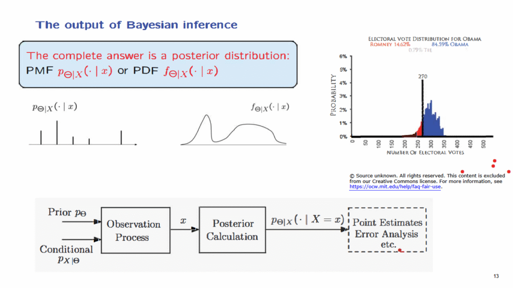
Or if Theta is continuous, a complete solution might be in the form of a conditional PDF that again tells us the conditional distribution of Theta.
To appreciate the idea here, consider the problem of guessing the number of electoral votes that a candidate gets in the presidential election.
The electoral votes are certain votes that the candidate gets from each one of the states in the United States.
And there is a certain number that the candidate needs to get in order to be elected president.
One possible prediction could be a statement that I predict that candidate A will win, but actually a more complete presentation of the results of a poll could be a diagram of this kind, which is essentially a PMF.
Here, a particular pollster collected all the data and gave the posterior probability distribution for the different possible numbers of electoral votes.
And this diagram is a lot more informative than the simple statement that we expect a certain candidate to get more than the required electoral votes.
So what is next?
As we just discussed, the complete solution is in terms of a posterior distribution, but sometimes, you may want to summarize this posterior distribution in a single number or a single estimate, and this could be a further stage of processing of the results.
So let us talk about this.
Once you have in your hands the posterior distribution of Theta, either in a discrete or in a continuous setting, and if you’re asked to provide a single guess about what Theta is, how might you proceed?
In the discrete case, you could argue as follows.
These values of Theta all have some chance of occurring.
This value of Theta is the one which is the most likely, so I’m going to report this value as my best guess of what Theta is.
And using a similar philosophy, you could look at the continuous case and find the value of Theta at which the PDF is largest and report that particular value.
This particular way of estimating Theta is called the maximum a posteriori probability rule.

We already have in our hands the specific value of X, and therefore, we have determined the conditional distribution for Theta.
What we then do is to find the value of theta that maximizes over all possible thetas the conditional PMF of this random variables capital Theta.
And similarly in the continuous case, the value of theta that maximizes the conditional PDF of the random variable Theta.
This is one way of coming up with an estimate.
One can think of other ways.
For example, I might want to report instead, the mean of the conditional distribution, which in this diagram might be somewhere here, and in this picture, it might be somewhere here.
This way of estimating theta is the conditional expectation estimator.
It just reports the value of the conditional expectation, the mean of this conditional distribution.
It is called the least mean squares estimator, because it has a certain useful and important property.
It is the estimator that gives you the smallest mean squared error.
We will discuss this particular issue in much more depth a little later.
Now, let me make two comments about terminology.
What we have produced here is an estimate.
I gave you the conditional PDF or conditional PMF, and you tell me a number.
This number, the estimate, is obtained by starting with the data, doing some processing to the data, and eventually, coming up with a numerical value.
Now, g is the way that we process the data.
It’s a certain rule.
Now, if we know the value of the data, we know what the estimate is going to be.
But if I do not tell you the value of the data and you look at the situation more abstractly, then the only thing you can tell me is that I will be seeing a random variable, capital X, I will do some processing to it, and then I will obtain a certain quantity.
Because capital X is random, the quantity that I will obtain will also be random.
It’s a random variable.
This random variable, capital Theta hat, we call it an estimator.
Sometimes, we might also use the term estimator to [refer to] the function g, which is the way that we process the data.
In any case, it is important to keep this distinction in mind.
The estimator is the rule that we use to process the data, and it is equivalent to a certain random variable.
An estimate is the specific numerical value that we get when the data take a specific numerical value.
So if little x is the numerical value of capital X, in that case, little theta hat is the numerical value of the estimator capital Theta hat.
So at this point, we have a complete conceptual framework.
We know, abstractly speaking, what it takes to calculate conditional distributions, and we have two specific estimators at hand.
All that’s left for us to do now is to consider various examples in which we can discuss what it takes to go through these various steps.