Introduction
In this segment we revisit the concept of conditional expectation and view it as an abstract object of a special kind.
To get going, let us start with something simple, the concept of a function.
Let’s say a function h that maps real numbers to real numbers.
As a concrete instance, consider the quadratic function that maps a number x to its square.
Consider now a random variable, capital X.
What do we mean when we write h of X?
For h defined– for example in this particular way as a quadratic function– h of X is defined to be a random variable.
Random Variable
Which random variable?
It is the random variable that takes the value little x squared whenever capital X, the random variable, happens to take the value little x.
And this is the random variable that we usually denote as the random variable X squared.
Now let this come to conditional expectations.
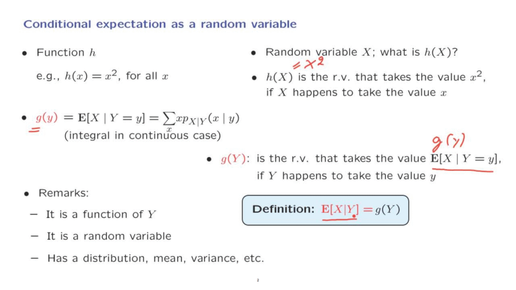
The conditional expectation of a discrete random variable is defined by this formula.
It is like the ordinary expectation except that we now live in a conditional universe in which the random variable capital Y is known to have taken a value little y.
And therefore, instead of using the ordinary formula for expectations that involve the PMF of X, we now use that formula but with the conditional PMF of X, which is the appropriate PMF that applies to this conditional universe.
Quantity
And if it happens that the random variable capital X is continuous, we would have an alternative formula but of the same kind, where the summation is replaced by an integral and the PMF is replaced by a PDF.
Now let us look at this quantity here.
We have fixed some particular little y.
Calculate this quantity.
And what we get is a number.
It is a number, but the value of that number depends on the choice of little y.
If I give you a different little y then you will get another number for this conditional expectation.
This means that this quantity here is really a function of little y.
And let us give a name to this function.
Let us call this function g.
Now that we have defined g we can ask, what is this object?
It’s a function of capital Y.
It’s a function of a random variable.
So it should be a random variable by itself.
By analogy, with the earlier concrete example, it is the random variable that takes the numerical value g of little y whenever capital Y happens to take the value little y.
But g of little y has been defined to be the same as this conditional expectation.
So it’s the random variable whose value is this conditional expectation, which is a particular number, if capital y happens to take the value little y.
This particular random variable that we have defined here, g of capital Y, we call it the abstract conditional expectation of the random variable X, given the random variable Y.
To summarize, this notation here stands for a random variable.
It is the random variable whose numerical value turns out to be this one if the value of the random variable capital Y happens to be little y.
It is a function of capital Y.
Once we know the value of capital Y, then the value of the conditional expectation is well defined.
It is known.
And it’s equal to this particular number.
It is of course a random variable.
And as a random variable, it has all the attributes that random variables have.
For example, it has a distribution, that is, a PMF or a PDF.
It has a mean of its own.
And it has a variance of its own.
So what will be next in our agenda is to talk about these attributes of this special random variable, and also to use it in several examples.