The covariance between two random variables tells us something about the strength of the dependence between them.
But it is not so easy to interpret qualitatively.
For example, if I tell you that the covariance of X and Y is equal to 5, this does not tell you very much about whether X and Y are closely related or not.
Another difficulty is that if X and Y are in units, let’s say, of meters, then the covariance will have units of meters squared.
And this is hard to interpret.
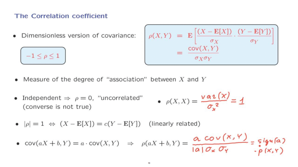
A much more informative quantity is the so-called correlation coefficient, which is a dimensionless version of the covariance.
It is defined by this formula here.
We just take the covariance and divide it by the product of the standard deviations of the two random variables.
Now, if X has units of meters, then the standard deviation also has units of meters.
And so this ratio will be dimensionless.
And it is not affected by the units that we’re using.
The same is true for this ratio here, and this is why the correlation coefficient does not have any units of its own.
One remark– if we’re dealing with a random variable whose standard deviation is equal to 0– so its variance is also equal to 0– then we have a random variable, which is identically equal to a constant.
Well, for such cases of degenerate random variables, then the correlation coefficient is not defined, because it would have involved a division by 0.
A very important property of the correlation coefficient is the following.
It turns out that the correlation coefficient is always between minus 1 and 1.
And this allows us to judge whether a certain correlation coefficient is big or not, because we now have an absolute scale.
And so it does provide a measure of the degree to which two random variables are associated.
To interpret the correlation coefficient, let’s now look at some extreme cases.
Suppose that X and Y are independent.
In that case, we know that the covariance is going to be equal to 0.
And therefore, the correlation coefficient is also going to be equal to 0.
And in that case, we say that the two random variables are uncorrelated.
However, the converse statement is not true.
We have seen already an example in which we have zero covariance and therefore zero correlation, but yet the two random variables were dependent.
Let us now look at the other extreme, where the two random variables are as dependent as they can be.
So let’s look at the correlation coefficient of one random variable with itself.
What is it going to be?
The covariance of a random variable with itself is just the variance of that random variable, now, sigma X is going to be the same as sigma Y, because we’re taking Y to be the same as X.
So we’re dividing by sigma X squared.
But the square of the standard deviation is the variance.
So we obtain a value of 1.
So a correlation coefficient of 1 shows up in such a case of an extreme dependence.
If instead we had taken the correlation coefficient of X with the negative of X, in that case, we would have obtained a correlation coefficient of minus 1.
A somewhat more general situation than the one we considered here is the following.
If we have two random variables that have a linear relationship– that is, if I know Y I can figure out the value of X with absolute certainty, and I can figure it out by using a linear formula.
In this case, it turns out that the correlation coefficient is either plus 1 or minus 1.
And the converse is true.
If the correlation coefficient has absolute value of 1, then the two random variables obey a deterministic linear relation between them.
So to conclude, an extreme value for the correlation coefficient of plus or minus 1 is equivalent to having a deterministic relation between the two random variables involved.
A final remark about the algebraic properties of the correlation coefficient- What can we say about the correlation coefficient of a linear function of a random variable with another?
Well, we already know something about what happens to the covariance when we form a linear function.
And the covariance of aX plus b with Y is related this way to the covariance of X with Y.
Now, let us use this property and calculate the correlation coefficient between aX plus b and Y.
In the numerator, we have the covariance of aX plus b with Y, which is equal to a times the covariance of X with Y.
At the denominator, we have the standard deviation of this random variable.
Now, the standard deviation of this random variable is equal to a times the standard deviation of X, if a is positive.
If a is negative, then we need to put the minus sign.
But in either case, we will have here the absolute value of a times the standard deviation of X.
And then we divide by the standard deviation of the second random variable, which is Y.
And so what we obtain here is this ratio, which is a correlation coefficient of X with Y times this quantity, which is the sign of a.
So we have the sign of a times the correlation coefficient of X with Y.
So in particular, the magnitude of the correlation coefficient is not going to change when we replace X by aX plus b.
And this essentially means that if we change the units of the random variable X, for example, suppose that X was degrees Celsius and aX plus b is degrees Fahrenheit, going from one set of units, Celsius degrees, to another set of units, degrees in Fahrenheit, is not going to change the correlation coefficient of the temperature with some other random variable.
So this is a nice property of the correlation coefficient, again, which reflects the fact that it’s dimensionless, it doesn’t have any units of its own, and it doesn’t depend on what kinds of units we use for each one of the random variables.