We now develop a methodology for finding the PDF of the sum of two independent random variables, when these random variables are continuous with known PDFs.
So in that case, Z will also be continuous and so will have a PDF.
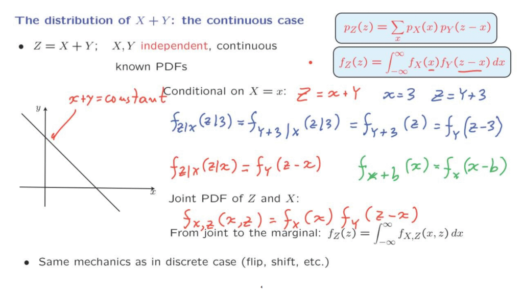
The development is quite analogous to the one for the discrete case.
And in the discrete case, we obtained this convolution formula.
This convolution formula corresponds to a summation over all ways that a certain sum can be realized.
In this picture, these are all the ways that the sum of 3 can be realized.
In the continuous case, the different ways that the constant sum can be realized corresponds to a line.
So this is a line in which X plus Y is equal to a constant.
And we need to somehow add over all the possible ways that the sum can be obtained, add over all the points on this line.
Now, when we’re summing over all the points of the line we really need to employ an integral.
And this leads to the following guess for the formula.
Instead of having a summation, we will have an integral.
And the integral is over all the X, Y pairs whose sum is a constant number, little z.
So we have here the family recipe– that sums are replaced by integrals and PMFs are replaced by PDFs.
So this formula is entirely plausible.
And it is called the continuous convolution formula.
What we want to do next is to actually justify this formula more rigorously.
We will use the following trick.
We will first condition on the random variable X, taking on a specific value.
If we do this conditioning, then the random variable Z becomes little x plus Y.
And to make the argument more transparent, we’re going to look first at the special case where little x is let’s say, the number 3.
In which case our random variable Z is equal to Y plus 3.
Let us now calculate the conditional PDF of Z in a universe in which we are told that the random variable X takes on the value of 3.
Now, given that X takes on the value of 3, the random variable Z is the same as the random variable Y plus 3.
And now we have the conditional PDF of y plus 3 given X.
However, we have assumed that X and Y are independent.
So the conditional PDF is going to be the same as the unconditional PDF of Y plus 3.
And we obtain this expression.
Now, what is this?
We know the PDF of Y.
But now we want the PDF of Y plus 3, which is a simple version of a linear function of a single random variable Y.
For a linear function of this form, we have already derived a formula.
In the notation we have used in the past, if we have a random variable X, and we add the constant to it, the PDF of the new random variable is the PDF of X but shifted by an amount equal to b to the right.
And that’s what the shifting corresponds to mathematically.
Now, let’s us apply this formula to the case that we have here.
We need to keep track of the different symbols.
So capital Y corresponds to X, b corresponds to 3, little x corresponds to Z.
And by using these correspondences, what we obtain is f sub Y of this argument, which is Z in our case minus b, which is 3 in our case.
And this is the final form for the conditional density of Z given that X takes a specific value.
It’s nothing more than the density of Y, but shifted by 3 units to the right.
Let us now generalize this.
Instead of using X equal to 3, let us use a general number.
And this gives us the more general formula, that the conditional PDF of Z given that X takes on a specific value is equal to– just use little x here instead of 3.
It takes this form.
So we do have now in our hands a formula for the conditional density of Z given X.
Since we have the conditional, and we also know the PDF of X, we can use the multiplication rule to find the joint PDF of X and Z.
By the multiplication rule, it is the marginal PDF of X times the conditional PDF of Z given X, which in our case takes this particular form.
And now that we have the joint PDF in our hands, we can use another familiar formula that takes us from the joint to the marginal.
It would take the joint PDF and integrate with respect to one argument, we obtain the marginal PDF of the other random variable.
Using this specific form that we have for the joint PDF in this formula, we have finally obtained this expression.
This is the integral of the joint PDF of X with Z integrated over all xs.
And this proves this convolution formula.
In terms of the mechanics of carrying out the calculation of the convolution, the mechanics are exactly the same as in the discrete case.
If you want to solve a problem graphically, what you will do is to take the PDF of Y, flip it horizontally, and then shift it by an amount of little z, cross multiply terms, and integrate them out.